
1. Financial Intermediation and the Banking System
A financial system connects decisions about saving, investment, borrowing and payment. A household may want to preserve purchasing power for retirement, a business may need funds before it can produce and sell its output, and a government may finance infrastructure whose benefits extend over decades. These plans rarely coincide in amount, timing or willingness to bear risk. Financial markets and intermediaries make them more compatible by creating claims, producing information, allocating risk and operating the infrastructure through which money and securities move. Their economic contribution depends on how well they perform these tasks, not simply on the volume of transactions they process.
Banking has both a developmental and a stability dimension. The 2006 Nobel Peace Prize awarded to Muhammad Yunus and Grameen Bank recognised the connection between access to finance and development from below. The 2022 economics prize awarded to Ben Bernanke, Douglas Diamond and Philip Dybvig recognised research on banks and financial crises. These perspectives belong together: institutions that expand access to useful finance can also become fragile when their promises to savers are easier to redeem than their assets are to realise.
How finance contributes to the real economy
Finance can improve production by moving resources toward projects that can use them productively. Mobilising savings allows investments larger than any individual saver could finance. Screening helps distinguish a viable enterprise from an implausible proposal. Monitoring gives the provider of funds an opportunity to detect diversion, excessive risk taking or deteriorating performance. Risk sharing permits investment that a single undiversified household might reject. Payments and settlement enable the resulting goods, services and financial claims to be exchanged reliably. These mechanisms explain why financial development can support economic development even when it does not increase the economy's aggregate saving rate.
There is also a direct household benefit through consumption smoothing. Income and desired expenditure need not occur in the same year. A student may borrow while studying and repay from later earnings; a worker may save during employment and consume those savings in retirement. Insurance transfers resources toward adverse states, such as illness or property damage. The relevant improvement is not a licence to spend without limit: borrowing remains constrained by future repayment capacity, while insurance requires sustainable pricing and incentives. Well-designed finance changes the timing and distribution of consumption without eliminating the economy's resource constraint.
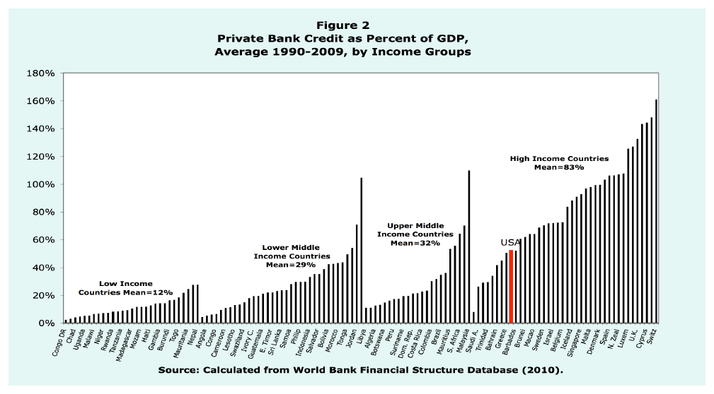
Historical comparisons show much higher private bank credit relative to GDP in many high-income economies than in low-income economies. In the 1990–2009 comparison below, the reported group means are approximately 12% for low-income countries, 29% for lower-middle-income countries, 32% for upper-middle-income countries and 83% for high-income countries. The dispersion within each group is substantial. These numbers describe an association, not a controlled experiment: income may increase the demand for sophisticated finance, effective institutions may encourage both development and lending, and credit may itself support investment. A causal interpretation needs a research design capable of distinguishing these channels.
Capital allocation and the limits of financial expansion
Capital allocation concerns which firms and projects obtain resources, rather than only how many resources are available. If two otherwise comparable firms face very different financing constraints, the more productive firm may remain too small while the less productive firm retains capital. Aggregate output can then be lower than it would be under a more efficient allocation. Financial information, collateral arrangements, legal enforcement and competition all influence this process, but they are not the only sources of distortion: taxation, product-market restrictions, management and technology also matter.
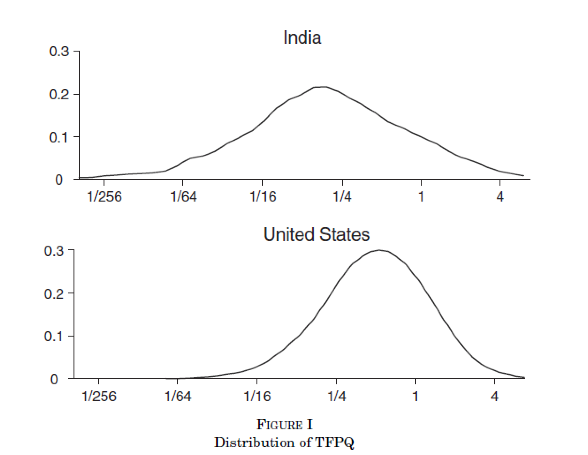
The manufacturing-productivity distributions reproduced below motivate the study of such differences. Physical total factor productivity, abbreviated TFPQ, measures output relative to an input bundle under the study's production assumptions. The distributions for India and the United States differ in location and shape. A distribution of physical productivity alone is not proof that lending is misallocated; the allocation argument requires examining how inputs are distributed across plants and how marginal products differ. Hsieh and Klenow's research uses establishment-level data to investigate these distortions. Its contribution is therefore more precise than the claim that a larger financial sector automatically causes higher productivity.
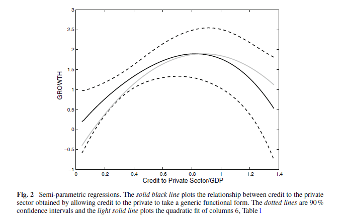
More finance can eventually produce diminishing benefits or accompany worse outcomes. Credit that funds a productive business is economically different from credit that finances a self-reinforcing increase in the price of existing property. A lending boom can relax collateral constraints, raise asset prices, encourage further borrowing and concentrate exposures to the same underlying risk. Resources may also be drawn into financial activities whose private returns exceed their contribution to aggregate production. The important question is whether additional intermediation improves information and investment decisions after allowing for the risks it creates.
The estimated finance–growth relationship below is nonlinear: in this historical sample, growth first rises and later falls as private credit relative to GDP increases. The dashed confidence limits indicate estimation uncertainty. The turning point is not a universal legal limit for an appropriate banking-sector size, and the fitted curve should not be treated as a forecast for a particular country. Results depend on the sample, controls, definition of credit, type of finance and period examined. Nor does a negative relationship at high credit levels establish that every additional loan is harmful; productive financing needs can remain unmet in an economy with a large aggregate banking system.
Research context: Hsieh and Klenow, Misallocation and Manufacturing TFP in China and India (2009); Arcand, Berkes and Panizza, Too Much Finance? (2015). The historical exhibits retain their original definitions and estimation periods.
Financial fragility and the wider cost of banking crises
A financial institution may create private profit while accumulating exposures that later impose costs on customers and the wider economy. Weak underwriting can expand credit in the short run, but losses eventually reduce banks' capacity or willingness to lend. Falling collateral values make refinancing harder; borrowers cut expenditure; investment and employment weaken; further defaults then damage bank balance sheets. The social cost of a crisis consequently extends beyond the losses borne by shareholders of the institutions that fail.
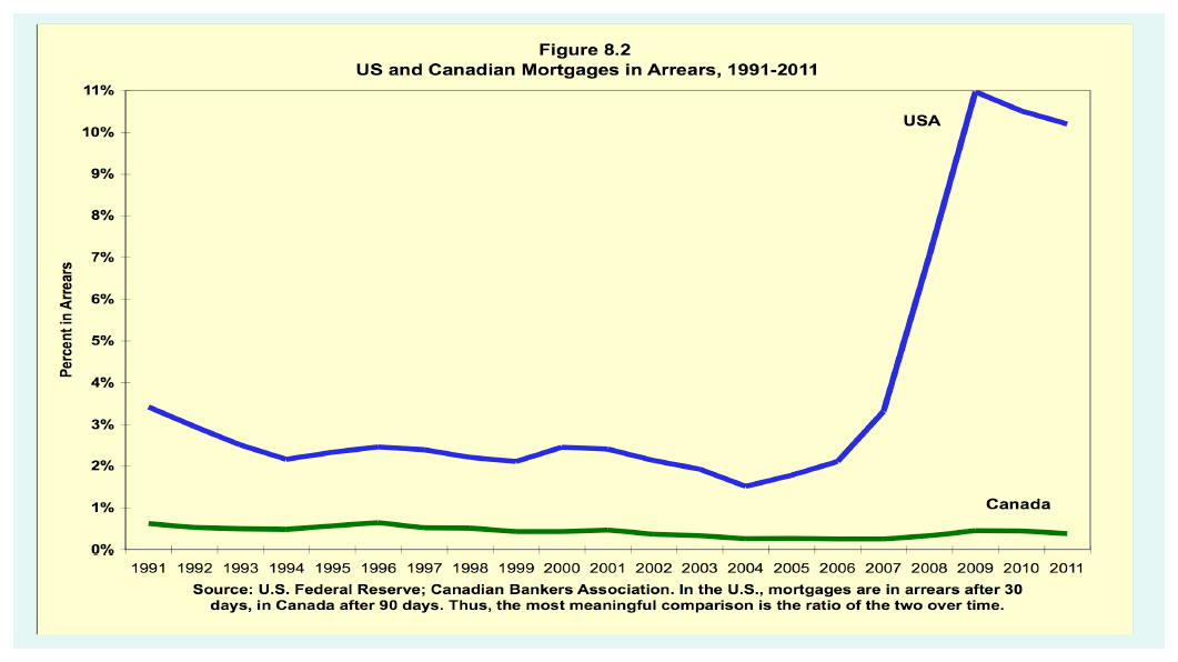
The US–Canada mortgage comparison illustrates the importance of both institutions and measurement. US arrears rose sharply around the global financial crisis, whereas the Canadian series remained much lower and more stable. However, the chart measures US mortgages after 30 days of arrears and Canadian mortgages after 90 days. It is therefore inappropriate to read the vertical gap as a like-for-like default-rate difference. The divergence over time is informative, but any explanation must also consider underwriting standards, mortgage contracts, housing-market conditions and the different arrears definitions.
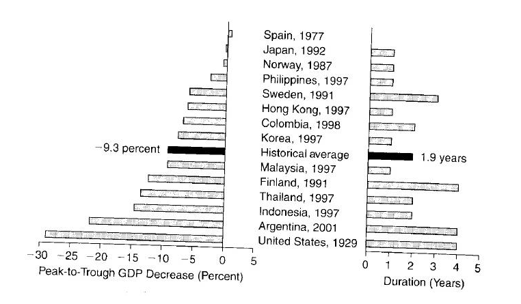
Historical crisis comparisons show substantial declines in output and long recoveries. In the selected episodes illustrated below, the reported average peak-to-trough real GDP decline is 9.3%, with a downturn lasting about 1.9 years. Related historical averages include unemployment increases of roughly seven percentage points, equity-price declines of about 56% and house-price declines of about 36%. These are summaries of selected past crises, not mechanical consequences of every bank failure. Different outcome measures may use different samples and time windows, so they should not be combined into a single representative country trajectory.
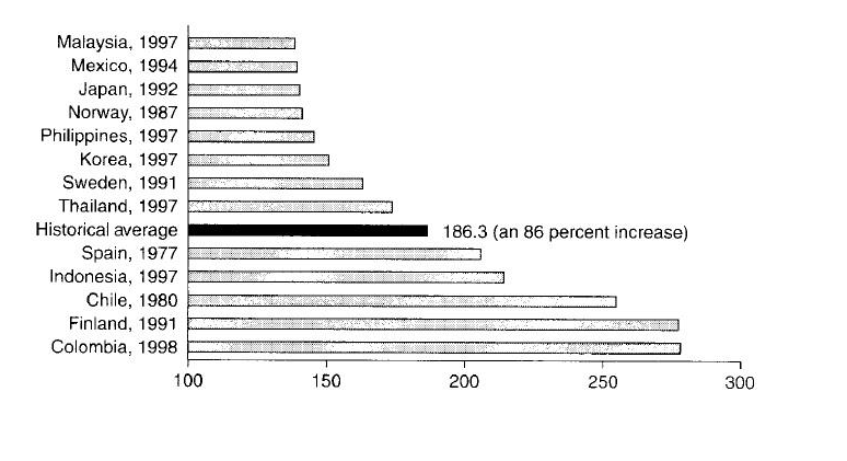
Public debt often increases after a crisis because tax receipts fall, automatic stabilisers support households, governments undertake discretionary measures and, in some cases, public resources support the financial system. The debt exhibit indexes the initial real debt level to 100; an average subsequent index of 186.3 means an increase of 86.3% in the real stock of debt. It does not mean an increase of 86.3 percentage points in the debt-to-GDP ratio, which has a different denominator. A deteriorating denominator can nevertheless make that ratio rise as well.
The problems are not confined to the distant past. Silicon Valley Bank and Signature Bank failed in the United States in March 2023, while Credit Suisse was taken over by UBS through an emergency transaction. Their circumstances differed, but they underline why funding concentration, asset values, confidence and access to liquidity must be assessed jointly. A bank can be vulnerable even when the assets it holds are not the same as those at the centre of the previous crisis. Later chapters develop the distinction between insolvency, illiquidity, contagious runs and the public interventions used to contain them.
Finance, wages and inequality
Financial development also affects the distribution of income. The historical US series below show that relative wages and the educational intensity of employment in finance changed markedly over the twentieth century. Both were high in the early decades, lower during much of the middle of the century, and rose again toward the end of the sample. The two series use different vertical scales: a movement in the education series cannot be read as the same percentage change as a movement in relative wages.
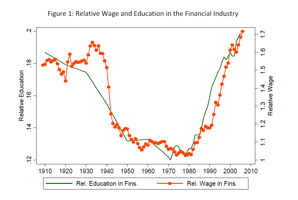
A wage premium may reflect specialised skills, demanding responsibilities, compensation for uncertain income or economic rents associated with market power and regulation. The chart alone does not identify their respective contributions. Likewise, finance may reduce inequality by widening access to credit and insurance while increasing inequality through high remuneration at the top of the sector or unequal access to profitable investment opportunities. Evaluating the distributional effect therefore requires examining who receives financial services, who bears losses and who captures the income generated by intermediation.
Direct finance, intermediated finance and the claims investors hold
A surplus unit has resources available beyond its current expenditure plans; a deficit unit seeks resources beyond its current income or internal funds. Financial markets connect them through securities. In direct finance, the ultimate investor holds a claim issued by the ultimate borrower: for example, a household or fund buys a company's bond, or an investor acquires newly issued shares. In indirect finance, an intermediary holds the claim on the borrower and issues a different claim to its own funders. A depositor has a claim on the bank, while the bank has a loan claim on a business.
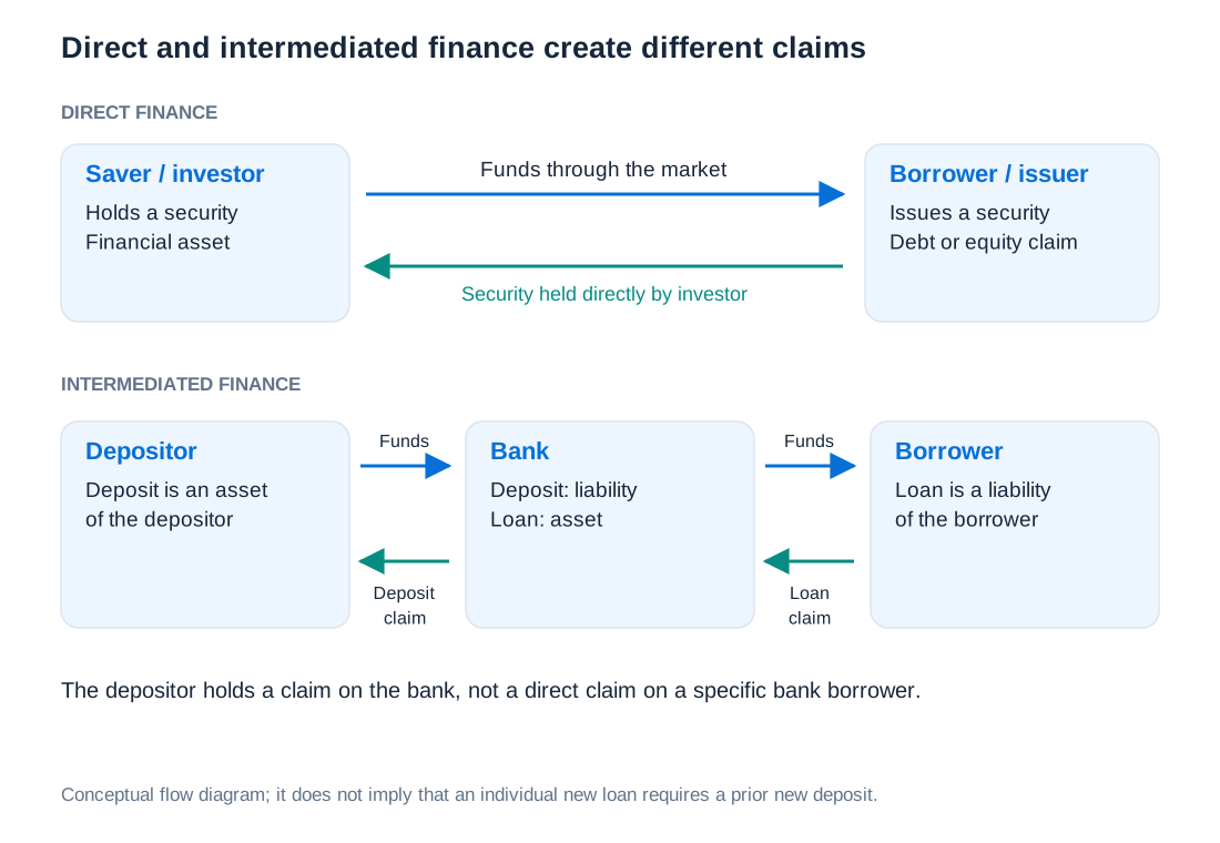
The presence of an intermediary in arranging a transaction does not automatically make the financing indirect in the balance-sheet sense. An investment bank can place a bond with investors while the investors remain creditors of the corporate issuer. A mutual fund pools investors' resources and purchases securities; investors generally bear changes in the value of the fund's portfolio through its net asset value. A commercial bank instead promises repayment of deposits according to their contractual terms even though the borrowers it finances may default. These arrangements differ in risk bearing, redemption rights and information production.
Insurance companies and pension institutions also channel saving into financial assets, typically against longer-horizon obligations. Investment companies, hedge funds and financial-technology businesses provide further combinations of management, matching, risk bearing and transaction services. Legal labels alone are not enough to classify a business. The analyst should ask whose balance sheet carries the exposure, who owes repayment to whom, whether a nominal value is promised and how withdrawal or redemption is funded.
The allocation-of-savings description should not be mistaken for a claim that a bank can lend only after locating an identical amount of pre-existing deposits. A bank can create a deposit when it grants a loan. It still needs capital, an economically viable borrower and a way to finance and settle payments when the newly created balance leaves the institution. The distinction between money creation and funding is developed in the chapter on money; it is already important here because intermediation is more than physically transferring a fixed stock of currency from one saver to one borrower.
Comparing the euro-area and US financial systems
The balance between banks and securities markets differs across economies. The December 2024 exhibits below portray a larger relative role for bank balance sheets in the euro area and a larger role for equity markets and pension funds in the United States. The first compares dollar amounts, while the second scales the aggregates by nominal GDP. Scaling matters: a larger economy can have larger financial markets in currency terms even if those markets are smaller relative to its annual output.
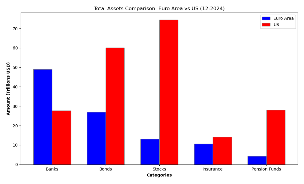
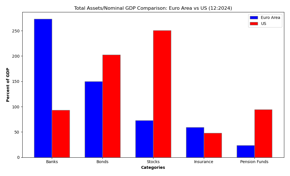
These categories are not mutually exclusive components of a single total. A bank may own bonds, an insurer may own shares, and a pension fund may hold claims on an investment fund. Adding bank assets, bonds, stock-market capitalisation, insurance assets and pension assets therefore double-counts many underlying claims. Moreover, securities outstanding and an institution's total assets are conceptually different aggregates. Exchange rates affect the dollar comparison; national accounting boundaries and consolidation rules affect both comparisons. The exhibits are historical structural illustrations, rather than a substitute for a harmonised financial-accounting dataset.
A bank-oriented system is not inherently superior or inferior to a market-oriented system. Banks can develop private borrower information and negotiate flexible contracts; markets can distribute risk widely and provide transparent prices for standardised claims. In practice they complement one another. A company can borrow from banks, issue bonds and sell equity, while the banks themselves use markets to obtain funding, hedge risks and distribute exposures.
Brokerage and information before a contract
The first core service of an intermediary is brokerage: bringing together parties with complementary needs and helping them transact. In the strict economic sense, a broker acts as an agent rather than purchasing the underlying exposure for its own account. A dealer, by contrast, takes a principal position. The same securities firm may perform both roles in different transactions. Calling an institution a broker consequently does not establish that all of its activities are free of balance-sheet risk.
Brokerage can overcome adverse selection, an information problem present before a contract is signed. A seller may know more about an asset's quality than a prospective purchaser; a borrower may know more about repayment prospects than a lender. If the less-informed party offers terms based on average quality, good-quality counterparties may find the terms unattractive, worsening the mix of those who participate. Screening, reliable disclosure and reputation can help investors distinguish among opportunities rather than pricing every transaction as though it were identical.
A retail investor choosing among investments, a bondholder evaluating an issuer's creditworthiness and an investor considering an initial public offering all confront this problem in different forms. A wealth manager can investigate investments and construct a suitable portfolio. A rating agency can produce a structured assessment of credit risk. An investment bank can organise due diligence, prepare offering documentation and explain the issuer to investors. None of these services guarantees a correct outcome; their value depends on the quality of the information and the incentives of the provider.
Specialisation also reduces duplicated screening. Suppose 100 investors would each spend EUR 200 producing substantially the same assessment of an issuer. Their combined research cost would be EUR 20,000. If a specialist can produce and distribute an equally useful assessment for EUR 5,000 in total, coordination saves EUR 15,000 even if the specialist is no more technically capable than an individual investor. This constructed example isolates a cost saving; fees, conflicts of interest and the value of independent second opinions can reduce the benefit. The correct claim is that brokerage can add value even when investors possess the necessary skills, not that every intermediary is always beneficial.
Monitoring, moral hazard and reusable information
After a contract is signed, the information problem changes. Moral hazard arises when a party's subsequent actions are difficult to observe or constrain and some consequences fall on another party. An insured firm may take less care to prevent damage; a manager may pursue acquisitions that increase personal power while reducing shareholder value; a borrower may shift toward a riskier project after receiving a loan. The defining feature is hidden or imperfectly controlled behaviour after contracting, rather than hidden borrower quality before contracting.
Monitoring responds to this problem by gathering information about actions and outcomes. Shareholders may use specialist advice when exercising voting rights. Lenders can require financial reports and covenants, investigate deterioration and negotiate corrective action. A portfolio manager may reduce exposure to issuers whose behaviour becomes inconsistent with the client's objectives. Selling a security does not itself remove the issuer's risk from the financial system, but the possibility of losing access to funding can affect incentives. Monitoring is costly, and excessive duplication among investors can again waste resources.
Information has value across both clients and time. Cross-sectional reusability means that analysing one firm helps an intermediary assess another: a rating specialist familiar with insurance balance sheets need not relearn the business model for every insurer. Intertemporal reusability means that past interaction improves subsequent assessment: a bank that helped a company issue equity may understand its later bond issue better because it already knows the management, reporting systems and business risks. These economies help explain persistent financial relationships, but also create switching costs and potential market power. A relationship is valuable when accumulated knowledge improves decisions, not merely because it is old.
Qualitative asset transformation
The second core service is qualitative asset transformation, usually abbreviated QAT. An intermediary acquires assets with one set of characteristics and offers its funders claims with another. A residential mortgage may be large, last for decades, trade infrequently and expose its owner to default risk. A household depositor may want a small divisible balance, immediate payment access and limited exposure to any individual mortgage. The bank bridges these demands using a portfolio of assets, funding arrangements, liquidity reserves and loss-absorbing capital.
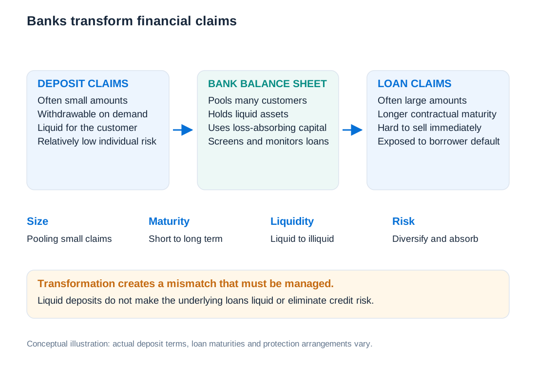
| Transformation | Mismatch the intermediary bridges | Economic implication |
|---|---|---|
| Size or lot size | Many small savings balances support larger loans | Pooling reduces minimum financing sizes and enables diversification |
| Maturity and repricing | Funding may mature or reprice before the assets it supports | Renewal risk and interest-rate risk arise when cash flows respond differently |
| Liquidity | Depositors can demand payment before loans can be sold at reasonable prices | Liquid buffers and reliable access to funding are necessary |
| Risk and conditionality | Risky asset cash flows support claims intended to be more predictable | Diversification, seniority and capital allocate losses rather than abolishing them |
| Currency | Assets and funding may be denominated in different currencies | Exchange-rate exposure and access to currency-specific liquidity require management |
Maturity and liquidity are related but distinct. A long-term bond can be readily marketable; a short-term private loan may be difficult to sell. Repricing maturity also differs from final maturity: a ten-year floating-rate loan may reset its interest rate frequently, whereas a shorter fixed-rate loan has a locked coupon until repayment. Identifying the relevant mismatch requires examining contractual cash flows and realistic customer behaviour, rather than assigning a single maturity number to every asset and liability.
Transformation inevitably places capital at risk. Diversification reduces exposure to an individual borrower's failure but does not eliminate a common recession or a market-wide liquidity shock. Depositors can hold relatively safe claims because losses initially fall on other stakeholders and because safeguards may apply; safety is not created by relabelling risky assets. Pure agency brokerage does not normally expose the intermediary to the customer's loan or market position, but it still involves operational, legal, conduct and reputational risks. The precise distinction is the absence or presence of the underlying principal exposure.
A worked distinction between liquidity and solvency
Consider a simplified institution holding EUR 85 of long-term loans and EUR 15 of immediately available liquid assets, financed by EUR 100 of deposits. Ignore equity only to isolate the liquidity arithmetic; a viable bank would ordinarily need a capital buffer. If depositors request EUR 40 at once, immediately available assets cover only EUR 15, leaving a EUR 25 funding gap. The loans might ultimately repay in full, yet the institution cannot meet the withdrawal without borrowing, selling assets or obtaining another source of liquidity. An inability to pay on time does not, by itself, establish that ultimate asset values are below liabilities.
Conversely, a bank can have enough cash to pay today's withdrawing depositors while the economic value of its remaining assets is less than its obligations. That is a solvency problem. A forced sale can connect the two: an initially solvent institution may realise large discounts while raising liquidity, reducing its equity and making doubts about solvency more credible. In a properly capitalised balance sheet, the first question is therefore whether asset values cover liabilities; the second is whether payment obligations can be met when due. Both need answers.
Payments, custody and the financial infrastructure
The third service is the operation of financial infrastructure. Cash services include access to ATMs and foreign-currency exchange. Transaction services include bank transfers, cheques and debit- or credit-card payments. Securities services include custody, clearing and settlement. Custody records and safeguards ownership; clearing establishes obligations between participants; settlement discharges those obligations through the final transfer of money or securities. These processes make finance usable in daily economic activity, including when the provider makes no loan to the customer.
Infrastructure produces risks of its own. A fault in ATM software can permit unauthorised withdrawals; a payment system may fail to execute instructions; a custodian may lose track of beneficial ownership or misuse client assets. Financial-crime and sanctions controls also matter because transaction networks connect counterparties across jurisdictions. These risks are not adequately measured by a loan default rate or an interest margin.
Two historical enforcement cases show the potential scale. In 2014, BNP Paribas agreed to plead guilty and pay approximately USD 8.9 billion in connection with processing transactions involving countries subject to US sanctions. In the MF Global case, US enforcement actions addressed misuse of segregated customer funds, with restitution obligations and monetary penalties. The economic lesson is that assets held for clients must remain distinguishable from the intermediary's own resources and that access to payment infrastructure carries legal responsibilities. Neither case is simply an example of ordinary borrowers failing to repay.
Historical case documentation: US Department of Justice, BNP Paribas agreement, 30 June 2014; CFTC, MF Global order, 24 December 2014. Prize context: Nobel Peace Prize 2006 and economics prize 2022.
These three services provide a practical way to analyse any financial institution. Ask first what information or matching service it supplies, then whether it transforms claims on its own balance sheet, and finally what infrastructure it operates. A universal bank may perform all three; a specialist platform may concentrate on one. The answers identify the sources of revenue, the risks that require management and the safeguards necessary to preserve the economic value of intermediation.
2. Bank Balance Sheets, Profitability and Performance
A bank's financial statements describe both the service it provides and the risks it accepts. A traditional lender holds loans and liquid assets against deposits and other funding. A broker may administer large customer portfolios while keeping little market exposure for its own account. A universal bank combines lending with wealth management, securities trading and other activities. The balance sheet shows the resulting stocks at a particular date; the income statement explains the flows of revenue, cost and profit over a period. Reading either statement in isolation can give a misleading impression of the institution.
This chapter develops a consistent method for interpreting these statements, then applies it to historical examples from Frankfurter Sparkasse, Trade Republic and UBS. The dates and accounting conventions are part of each example. Figures from different years or reporting frameworks are useful for comparing business models, but they are not a ranking of the institutions' current strength. The worked stress tests and strategy changes are constructed scenarios, not forecasts or statements about events that actually occurred.
Assets, liabilities and equity
Assets are economic resources or claims held by the bank. Cash and central-bank reserves support payments; securities can provide investment income and, depending on their characteristics, liquidity; loans generate contractual interest and principal payments from borrowers. Other assets may include property, equipment, receivables and intangible assets. Liabilities are obligations to outsiders, including customer deposits, interbank borrowing, issued debt and other payables. A customer deposit is an asset of the customer but a liability of the bank. Equity is the residual interest after recognised liabilities are deducted from recognised assets.
Let denote assets, liabilities and equity, all measured in the same currency at the same date. The accounting identity is
The identity must hold after every transaction. If a bank grants a EUR 10,000 loan and credits the customer's account, loan assets and deposit liabilities both rise by EUR 10,000. If the customer then pays someone at another bank, the originating institution loses the customer deposit and must deliver settlement resources to the receiving institution. The original loan remains on its balance sheet. Deposit creation and subsequent funding needs are compatible; the ability to create an accounting entry does not remove constraints on capital, credit quality or settlement liquidity.
Equity is not a pile of cash in a separate account. It is a funding claim and an accounting residual. A bank can invest resources financed by equity in illiquid loans, just as it can hold cash financed by deposits. This explains why a well-capitalised institution can face a liquidity shortage and why a cash-rich institution can still have insufficient asset value to cover its debts. The amounts at which assets appear in the accounts also depend on the relevant recognition and measurement rules. Book values, market values and regulatory exposure values need not coincide.
Leverage magnifies asset losses and shareholder returns
The accounting equity ratio is , while assets-to-equity leverage is . Consider assets of EUR 1,000 million, liabilities of EUR 950 million and equity of EUR 50 million. The equity ratio is 5% and leverage is 20 times. An impairment of EUR 20 million reduces assets to EUR 980 million. If liabilities remain EUR 950 million, equity falls to EUR 30 million: a 2% loss of assets has destroyed 40% of the initial equity. The change is not an additional cash payment by shareholders; it is the effect of the residual claim absorbing the asset loss.
If leverage had instead been 50 times, initial equity would have been only 2% of assets, and the same 2% asset loss would exhaust it. The calculation deliberately excludes taxes, new capital, profit earned during the period and any change in liabilities. It illustrates sensitivity rather than determining a regulatory capital requirement. A bank's capital adequacy also depends on the risks of its assets, off-balance-sheet commitments and the eligibility of its capital instruments.
Leverage also explains why return on equity can look high when return on assets is modest. With net income of EUR 10 million on EUR 1,000 million of assets and EUR 50 million of equity, return on assets is 1% and return on equity is 20%. Using the same profit numerator and consistent balance definitions,
Average balances are generally preferable when comparing a flow earned over the year with the resources used to earn it; year-end balances can be used for a simplified exercise if clearly identified. The identity is a decomposition, not proof that raising leverage creates economic value. Debt-funded expansion can increase funding costs and risk, while a reduction in equity makes the remaining shareholders more exposed to a given loss.
A deposit-and-loan bank: the Frankfurter Sparkasse example
Frankfurter Sparkasse illustrates a regional savings-bank model: it takes deposits, makes loans and holds assets that support payments and liquidity management. The simplified statement below groups its 2024 accounts into broad economic categories. The analytical equity amount includes the fund for general banking risks, so it is broader than a narrowly defined ordinary equity line in statutory accounts. It should not be identified automatically with common equity tier 1, or CET1, capital. The latter requires prudential eligibility tests and adjustments.
| Side | Item | Amount |
|---|---|---|
| Assets | Cash | 269 |
| Assets | Securities | 4,959 |
| Assets | Loans | 17,124 |
| Assets | Other assets | 372 |
| Assets | Total assets | 22,724 |
| Funding | Deposits | 21,171 |
| Funding | Other liabilities | 315 |
| Funding | Analytical equity, including general banking-risk fund | 1,238 |
| Funding | Total liabilities plus analytical equity | 22,724 |
Loans account for EUR 17,124 million of assets, but not all of them are household or corporate customer loans: EUR 6,203 million are claims on banks and EUR 10,921 million are customer loans. EUR 4,958 million of the customer-loan book is backed by real-estate collateral. Collateral can reduce loss severity but does not make a loan risk-free; its value and realisability matter when the borrower defaults. EUR 14,081 million of total loans have more than one year remaining to maturity, whereas EUR 16,050 million of deposits are overnight funding.
| Category | Component | Amount |
|---|---|---|
| Securities | Fixed-income instruments | 4,258 |
| Securities | Equity instruments | 701 |
| Securities | Total | 4,959 |
| Loans | Loans to banks | 6,203 |
| Loans | Loans to customers | 10,921 |
| Customer loans | Of which: real-estate collateral | 4,958 |
| Loans | Total | 17,124 |
| Total loans | Of which: remaining maturity over one year | 14,081 |
| Deposits | Overnight | 16,050 |
| Deposits | Other deposits, rounded | 5,122 |
| Deposits | Reported total | 21,171 |
The separately rounded overnight and other-deposit amounts add to EUR 21,172 million, whereas the reported deposit total is EUR 21,171 million. The reported total is used consistently in the ratios and scenarios.
The distinction between fixed-income securities and equities matters for stress analysis. The securities total is EUR 4,959 million, comprising EUR 4,258 million of fixed-income instruments and EUR 701 million of equities. A sovereign-default scenario applied to all fixed-income securities therefore uses EUR 4,258 million, not the entire securities portfolio. Similarly, a simple liquidity calculation that counts every security at its current carrying amount makes a strong assumption about saleability and prices; equities and long-duration bonds are not interchangeable with cash.
Historical accounting basis: Frankfurter Sparkasse, annual report 2024, regrouped and rounded for analysis. The fund for general banking risks is governed by section 340g of the German Commercial Code. Section 340e contains particular valuation and trading-book provisions; it is not the general statutory heading for this fund.
Funding and liquidity ratios need explicit denominators
The equity ratio expresses the size of the loss-absorbing accounting cushion. The loan-to-deposit ratio compares one main use of funds with one main source. The liquid-assets ratio measures the share of assets allocated to a specified liquid category. None is a complete risk assessment. Loans can be risky even when they are fully funded by deposits; a bank with a loan-to-deposit ratio below 100% can still experience a run; and securities classified as liquid in a simple accounting exercise may be encumbered or saleable only at a discount.
| Indicator | Calculation | Result | Interpretation |
|---|---|---|---|
| Analytical equity ratio | 1,238 / 22,724 | 5.45% | Accounting loss-absorption buffer relative to assets |
| Loan-to-deposit ratio | 17,124 / 21,171 | 80.88% | Loan volume relative to deposit funding |
| Simple liquid-assets ratio | (269 + 4,959) / 22,724 | 23.01% | Cash plus all securities relative to assets |
| Overnight funding / total funding | 16,050 / 22,724 | 70.63% | Funding denominator includes analytical equity |
| Overnight funding / liabilities | 16,050 / (22,724 − 1,238) | 74.70% | Funding denominator excludes analytical equity |
The overnight-funding ratio particularly requires care. Dividing EUR 16,050 million by total assets of EUR 22,724 million gives 70.63% of total funding including analytical equity. Dividing by liabilities excluding that equity, EUR 21,486 million, gives 74.70%. Both calculations can be informative, but they answer different questions. Labelling the first denominator “total liabilities” while including equity obscures the distinction. Nor does a non-overnight funding share guarantee that all remaining funding is unconditionally available under every stress: contractual options, collateral calls and other obligations may still matter.
A book equity ratio differs from a regulatory CET1 ratio, whose denominator is risk-weighted exposures rather than unweighted assets. A simple liquid-assets ratio also differs from the liquidity coverage ratio, which applies eligibility rules, haircuts and a defined 30-day stress to cash inflows and outflows. These regulatory measures are developed later. Here the purpose is to extract economically meaningful information from a simplified balance sheet while stating the limits of each measure.
From interest revenue to net profit
Interest income is the gross revenue earned from interest-bearing assets. Interest expense is the cost of interest-bearing funding. Their difference is net interest income, or NII. Fees and commissions reward services such as account administration, payments, investment distribution and advice. Trading results arise from market-making or other positions and can be volatile. Administrative expenses pay for staff, premises, technology and other operating resources. Credit-loss charges recognise deterioration in the expected collection of assets. Taxes and other separately reported items then determine the final profit.
| Item | Amount | Interpretation |
|---|---|---|
| Interest income (component) | 699.7 | Interest earned on loans, securities and other relevant assets |
| Interest expense (component) | −377.1 | Interest paid on deposit funding in the simplified presentation |
| Net interest income (reported subtotal) | 322.5 | Use this subtotal once in the profit bridge |
| Net fee and commission income | 121.0 | Account, transaction and related service revenue |
| Trading income | 0.0 | No material amount in this grouping |
| Credit-loss provisioning expense | −23.8 | Precautionary expense for increased risk of future loan losses |
| Salary and administrative expense | −295.9 | Personnel, premises, technology and other operating costs |
| Allocation to the general banking-risk fund | −40.0 | Separate HGB allocation, not a realised borrower default |
| Other income and costs, net | 33.8 | Remaining grouped items |
| Income before tax | 117.6 | Reported pretax result |
| Tax expense | −57.6 | Deduction from pretax result |
| Income after tax | 60.0 | Reported net result |
The EUR 23.8 million credit-loss charge is a precautionary expense accounting for increased risk of future loan losses. It is not a profit generated because a borrower previously expected to default suddenly repaid. A provision expense lowers profit; a release of an existing allowance normally has the opposite effect. The precise recognition and measurement rules depend on the applicable accounting framework. Under IFRS 9, expected-credit-loss accounting is forward-looking; the statutory German accounts in this historical example must nevertheless be understood under their own HGB framework, rather than silently replacing it with IFRS terminology.
The EUR 40 million allocation to the fund for general banking risks is separate from the credit-loss charge. It reduces the reported income available after that allocation but contributes to the broader analytical capital buffer used here. Treating it as an additional realised borrower default would therefore be misleading. Using the reported net interest income and the grouped items, the profit bridge is million before tax, and million after tax. The gross rounded interest amounts differ from the reported net interest subtotal by EUR 0.1 million; the reported subtotal is retained rather than forcing an artificial reconciliation.
For comparison, an entirely illustrative bank earning EUR 54 million of interest and paying EUR 26 million generates NII of EUR 28 million. Adding EUR 12 million of fees and deducting EUR 24 million of operating costs and EUR 8 million of credit-loss charges produces EUR 8 million before tax. If average interest-earning assets are EUR 1,400 million, its net interest margin is . This example separates the absolute amount of income from the rate earned on the underlying asset base.
Asset yields, funding costs and operating efficiency
The simplified average yield on cash, securities and loans in the Sparkasse example is . This denominator uses year-end amounts and includes cash, so the result is an analytical approximation rather than a contractual loan interest rate. The average interest expense on deposits is . Its denominator is deposits only, not deposits plus other liabilities. The difference is percentage points.
| Measure | Calculation | Result |
|---|---|---|
| Average asset yield, simplified | 699.7 / (269 + 4,959 + 17,124) | 3.13% |
| Average interest expense on deposits | 377.1 / 21,171 | 1.78% |
| Asset-yield minus deposit-cost spread | 3.13% − 1.78% | 1.35 percentage points |
| Cost-to-income ratio under the stated grouping | 295.9 / (322.5 + 121.0 + 0.0) | 66.72% |
| After-tax return on analytical equity | 60.0 / 1,238 | 4.85% |
This yield–cost spread is not identical to net interest margin. NIM divides net interest income by a defined asset base, commonly average interest-earning assets. Subtracting two rates calculated on different denominators is economically useful but is not an algebraic replacement for dividing net income by assets. Deposit service fees, non-interest-bearing balances, wholesale funding and the asset mix further complicate comparisons. A higher loan rate may compensate for expected defaults, illiquidity, origination expense or capital consumption instead of representing a pure increase in profit.
The cost-to-income ratio used here is , or about 66.7%. Operating expense therefore absorbs roughly two thirds of the specified revenue before the separately reported credit-loss charge and other items. Different institutions may include other operating income, treat restructuring costs differently or use another denominator. A lower ratio can indicate greater efficiency, but it can also result from temporarily buoyant trading income or insufficient investment in systems. A ratio only becomes comparable after its components are reconciled.
The after-tax return on analytical equity is . This does not imply that every shareholder or owner received a 4.85% cash distribution; accounting profit may be retained. Nor does it measure a market return, which also depends on the price paid for the equity and changes in that price. Profitability, payout and valuation are related but distinct concepts.
A brokerage model: Trade Republic in September 2023
The historical Trade Republic example captures a predominantly brokerage and transaction-service business before its full banking licence was announced in December 2023. At the September 2023 reporting date, customer cash in the simplified presentation was held through trust arrangements with partner banks. Calling these balances “deposits” for a business-model comparison must not imply that their legal treatment was identical to ordinary deposits funded directly on a traditional lender's balance sheet. The date is essential: this is not a description of all products or legal arrangements offered subsequently.
| Side | Item | Amount |
|---|---|---|
| Assets | Cash | 10 |
| Assets | Balances with banks, including customer trust arrangements | 6,966 |
| Assets | Other assets | 47 |
| Assets | Total | 7,023 |
| Funding | Customer cash shown as deposits in the simplified comparison | 6,411 |
| Funding | Other liabilities | 80 |
| Funding | Equity | 532 |
| Funding | Total | 7,023 |
The example reports approximately EUR 29 billion of assets under management and 3.5 million customers. Customer securities administered by a platform are not automatically assets owned by the platform. Consequently, the value of customer portfolios can greatly exceed the institution's own economic exposures. It is equally important not to conclude that the EUR 7,023 million presentation is entirely proprietary money: much of it reflects matched customer trust balances. Separating customer property, custodial responsibilities and the firm's own assets is necessary before measuring leverage or credit risk.
| Item | Amount | Interpretation |
|---|---|---|
| Interest income (component) | 10.2 | Interest received from partner banks on deposits |
| Interest expense (component) | 0.0 | No material amount in this grouping |
| Net interest income (subtotal) | 10.2 | Do not add this subtotal to its own components |
| Fee and commission income | 148.7 | Brokerage and transaction-related services |
| Trading income | 0.2 | Small own-account result |
| Credit-loss provision charge | 0.0 | No material lending business in this example |
| Salary and administrative expense | −135.4 | Staff, premises, IT and marketing |
| Other income and costs, net | −7.4 | Other grouped items |
| Income before tax (reported) | 16.2 | Rounded reported subtotal |
| Tax expense | −2.2 | Rounded tax charge |
| Income after tax (reported) | 14.1 | Rounded reported result |
The EUR 10.2 million interest income represents interest received from partner banks on deposits, not negative interest on bank deposits. Fees and commissions of EUR 148.7 million dominate the revenue mix, while the reported credit-loss charge is zero in this simplified historical model without material lending activity. Operating costs, including technology, staff and marketing, remain substantial. Small differences of EUR 0.1 million arise when rounded components are recomputed; the reported subtotals are preserved.
Lower direct lending exposure does not mean negligible business risk. Falling asset prices can reduce customer portfolio values and any fees linked to them. Trading activity, investor confidence and customer retention can change revenue. Outages, failed orders, misuse of assets, cyber incidents, inaccurate statements or weak compliance can cause direct expense and reputational damage. Partner-bank exposure and the precise safeguarding arrangements also matter. A stress analysis appropriate for a mortgage lender cannot simply be copied onto a broker.
Historical licence chronology: Trade Republic announcement of 6 December 2023. The financial illustration uses the reporting year ending 30 September 2023 and should be interpreted at that date.
A universal bank: UBS at the end of 2024
A universal bank combines several intermediation technologies. UBS's simplified 2024 statement contains loans and deposits alongside large derivative, trading and repurchase-agreement positions. A reverse repo is economically a collateralised cash-lending arrangement; a repo is collateralised funding. The exact accounting depends on the contract and applicable rules, but the distinction explains why similar securities can participate in different financing transactions. A short position creates an obligation associated with selling a security the institution must subsequently deliver or repurchase.
| Side | Item | Amount |
|---|---|---|
| Assets | Cash | 223.3 |
| Assets | Loans | 598.9 |
| Assets | Derivative assets | 185.6 |
| Assets | Trading assets | 159.1 |
| Assets | Reverse repos | 118.3 |
| Assets | Other assets | 279.9 |
| Assets | Reported total | 1,565.0 |
| Funding | Deposits | 745.8 |
| Funding | Other borrowed money | 214.2 |
| Funding | Derivative liabilities | 180.6 |
| Funding | Short positions | 35.2 |
| Funding | Repos | 14.8 |
| Funding | Other liabilities | 288.7 |
| Funding | Equity | 85.6 |
| Funding | Reported total | 1,565.0 |
The total of approximately USD 1.565 trillion indicates the scale of the group, but it is not itself a measure of expected losses. A derivative asset is generally the positive fair value of a contract, not its notional principal. Derivative liabilities may offset some market sensitivities, but gross accounting assets and liabilities cannot simply be netted without considering enforceable agreements, counterparties and collateral. Gross balance-sheet size, market risk, counterparty exposure and liquidity needs consequently provide different views of the same business.
| Item | Amount | Economic meaning |
|---|---|---|
| Interest income (component) | 43.1 | Interest on loans, deposits, repos, trading assets and other balances |
| Interest expense (component) | −35.9 | Cost of deposits, borrowing, repos, issued debt and other funding |
| Net interest income (reported subtotal) | 7.1 | Net interest contribution; use once in the earnings bridge |
| Credit-loss provisions | −0.6 | Expense for credit deterioration |
| Fee and commission income | 26.1 | Wealth-management and other service revenue |
| Trading income | 14.7 | Market-making and other trading results |
| Salary and administrative expense | −37.4 | Operating cost |
| Other income and expenses, net | −3.1 | Other grouped items |
| Income before tax | 6.8 | Pretax result |
| Tax expense | −1.7 | Deduction from pretax result |
| Income after tax | 5.1 | Net result |
Fees and commissions of USD 26.1 billion and trading income of USD 14.7 billion are central to this illustration, while net interest income is USD 7.1 billion. That combination differs substantially from a regional deposit-and-loan institution. The label “trading income” can include customer-driven market-making as well as proprietary risk; it should not be interpreted as pure speculation without examining the detailed accounts. Similarly, large administrative costs partly reflect the service-intensive nature of wealth management and the complexity of operating across markets.
Small rounding differences occur in the regrouped balance sheet and between rounded gross interest income and expense. They do not justify altering a published subtotal to make a teaching table add exactly. More fundamentally, a balance sheet and income statement alone cannot reveal the direction of every market sensitivity. Two banks with identical derivative asset values can react differently to an interest-rate shock because their contracts, maturities, hedges and collateral terms differ. Meaningful stress testing requires positions and cash flows at a much finer level of detail.
Interest-rate stress: earnings and market values are different channels
Consider a one-year earnings shock to the Sparkasse example. Assume market rates rise immediately by two percentage points, the increase is fully passed through to EUR 16,050 million of overnight deposits, other deposits and liabilities do not reprice, and all loans remain fixed rate for the year. Also assume cash and all securities earn the higher rate immediately, while no position changes market value. The last assumption is deliberately stylised: many fixed-rate bonds do not reprice their coupons, and an actual rate increase may reduce their market price.
Starting from pretax profit of EUR 117.6 million, the stressed result becomes a loss of EUR 98.84 million before tax. The incremental deterioration of EUR 216.44 million is 17.48% of initial analytical equity, while the stressed pretax loss itself is 7.98% of that equity. These are different quantities: describing the entire incremental shock as a fall in year-end capital while also subtracting the stressed loss would count the shock twice. Taxes, distributions and other changes in capital are excluded from this calculation.
The scenario illustrates a negative short-term repricing gap: rate-sensitive funding exceeds rate-sensitive assets. A lower deposit pass-through would reduce the earnings damage; variable-rate loans would increase the offsetting income response. In practice, deposit migration toward better-remunerated accounts can make funding costs rise even without a uniform increase on every account. Contractual repricing schedules, customer behaviour and hedges therefore determine the actual result.
A separate constructed example isolates the market-value channel. A fixed-income portfolio worth EUR 200 million has modified duration . For a parallel yield increase of 1.5 percentage points, the first-order estimate is
The minus sign reflects the inverse relationship between fixed-rate bond prices and yields. Modified duration is a local approximation, and 150 basis points is large enough that convexity can materially affect accuracy. The example excludes changes in credit spreads, optionality and cash flows. Whether and when such a value change affects reported profit or regulatory capital depends on the accounting classification and prudential treatment. An earnings stress and a market-value stress must therefore be specified separately before their results are combined.
Credit-loss and sovereign-risk stress
Suppose the bank must increase credit-loss provisions by 1% of its EUR 17,124 million loan book. The additional charge is million. Holding everything else constant, pretax profit becomes million. The incremental charge equals 13.83% of initial analytical equity. It is a charge against expected recoverability, not an assumption that EUR 171.24 million of cash necessarily leaves the bank that day. The provision can worsen solvency measures while having a different immediate liquidity effect.
Now assume, solely for a sovereign-risk scenario, that every EUR 4,258 million of fixed-income securities is a claim on one government, that default probability is 50%, recovery is zero and discounting is ignored. Expected repayment value falls to 50% of the initial exposure, implying a EUR 2,129 million loss under this simplified valuation. Initial equity of EUR 1,238 million is insufficient: subtracting that loss produces negative analytical equity of EUR 891 million. This is not an assertion that actual market prices always equal one minus a physical default probability; risk premia, timing, recovery and existing prices matter in a proper valuation.
The case shows how a concentrated government-bond portfolio can link bank and sovereign solvency. A weaker sovereign reduces the value of bank assets and possibly the credibility of public guarantees. Supporting banks can in turn increase sovereign financing needs, reinforcing the weakness. Domestic government securities can be attractive because of liquidity, collateral use, regulation and familiarity, but a strong concentration creates a common exposure rather than true diversification.
An institution can remain liquid for a time even after economic losses exhaust its capital, especially if losses are not promptly recognised or creditors do not withdraw. Continuing in that state can create incentives to “gamble for resurrection”: owners with little remaining value may prefer a high-risk strategy that benefits them if it succeeds while leaving much of the downside to creditors or public backstops. Prompt loss recognition and credible intervention address a solvency problem; an additional short-term loan alone cannot restore the missing asset value.
Deposit withdrawals and the remaining liquidity buffer
A run scenario asks how quickly the bank can meet withdrawals. Start with EUR 21,171 million of deposits and EUR 5,228 million of cash plus securities. Assume securities can be sold instantly at their stated values, are unencumbered and incur no transaction cost. These assumptions provide an upper-bound-style liquidity illustration, not a regulatory liquidity assessment. In a 20% withdrawal scenario, outflows are million, leaving million of liquid assets.
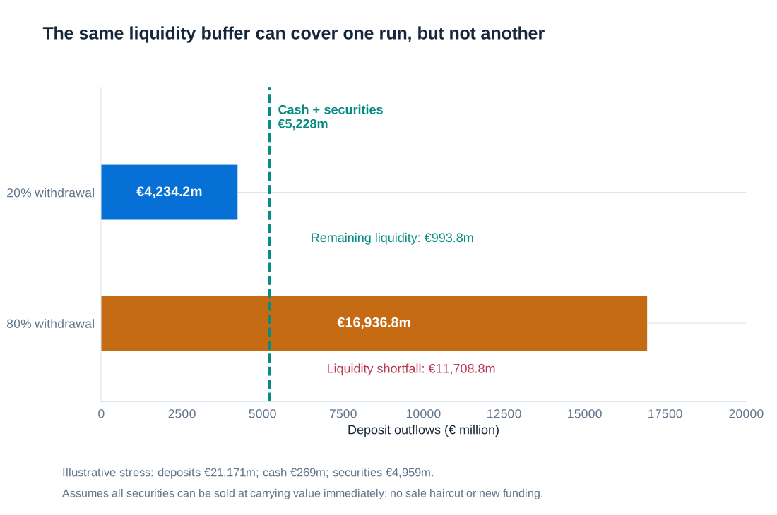
The immediate withdrawal can therefore be covered under these assumptions, but the institution is much less liquid afterwards. Its remaining deposit base is EUR 16,936.8 million, and, absent other changes, total assets shrink to EUR 18,489.8 million. Remaining liquid assets are only about 5.37% of that smaller balance sheet. Paying today's withdrawals is not sufficient if tomorrow's depositors view the depleted buffer as evidence that they should leave as well.
An 80% withdrawal instead requires million. Available cash and securities leave a shortfall of EUR 11,708.8 million. The bank would need additional funding, loan sales, collateralised borrowing or another source of liquidity to meet the scenario. Such options cannot be assumed costless or certain. Haircuts, unavailable collateral and simultaneous stress at other institutions can make the gap larger. Failure to pay under this scenario demonstrates illiquidity under the assumed resources; whether the bank is also insolvent requires an assessment of asset values and losses.
The same stresses affect different business models differently. A broker with matched customer cash arrangements and little lending can have a smaller direct sensitivity to loan losses, but falling markets, partner-bank problems and loss of customer confidence can damage its revenue or operations. A universal bank's derivatives and trading positions may either hedge or amplify rate and market shocks. Opaque asset positions make creditors uncertain about where losses lie, which can itself accelerate withdrawals. A useful stress test therefore specifies the shock, the balance-sheet transmission, behavioural assumptions and available management responses.
Strategy one: replacing equity with deposits
Consider three separate changes to the initial Sparkasse balance sheet. Each starts from the original amounts; they are not cumulative. To make the arithmetic transparent, assume the tax charge and all unmentioned income and expenses remain fixed. Incremental pretax earnings then change reported after-tax income euro for euro in this simplified exercise. This is an assumption about the calculation, not a realistic forecast of marginal taxation.
First replace EUR 200 million of equity funding with deposits while keeping total assets constant. Analytical equity falls from EUR 1,238 million to EUR 1,038 million and deposits rise to EUR 21,371 million. This can be understood as new deposit funding financing a distribution of capital. At the initial average deposit cost of , extra annual interest expense is approximately EUR 3.56 million. Profit falls from EUR 60 million to about EUR 56.44 million.
ROE has risen from 4.85% despite a reduction in total profit. The reason is that the equity denominator falls proportionately more than income. The change makes the institution more leveraged, reduces the buffer against asset losses and replaces permanent loss-absorbing funding with a claim that may be withdrawable. A higher ROE therefore does not establish that the bank has become more efficient or created more value after adjusting for risk.
Strategy two: replacing securities with loans
Next replace EUR 1 billion of securities with loans that earn one percentage point more. Assume, for the comparison, that both the old securities and new loans are free of credit losses. Total assets, deposits and analytical equity remain unchanged. Loans increase to EUR 18,124 million and securities fall to EUR 3,959 million. Incremental annual interest income is million, so profit rises to EUR 70 million under the fixed-tax assumption.
The loan-to-deposit ratio rises from 80.88%, while the liquid-assets ratio falls from 23.01%. These values use the same 2024 balance sheet throughout. The strategy improves the assumed earnings yield by reducing liquidity. It does not create credit risk within an exercise that explicitly assumes both assets are credit-risk-free; in an actual implementation, differences in borrower risk, capital requirements, origination cost and maturity would need to be added. Even a loan certain to repay eventually can be hard to sell before maturity, so liquidity risk remains possible under the risk-free-credit assumption.
Strategy three: accepting more credit risk
Finally replace the entire EUR 17,124 million loan book with loans earning 100 basis points more but requiring 50 basis points more in annual credit-loss provisions. One hundred basis points equals one percentage point. Additional interest income is EUR 171.24 million and additional provisioning is EUR 85.62 million, leaving EUR 85.62 million of extra profit under the fixed-tax assumption. New profit is EUR 145.62 million and .
The average yield on cash, securities and loans rises to . With the same deposit cost of 1.78%, the simplified yield–cost spread becomes about 2.12 percentage points. This is a substantial increase in reported expected profitability, but the higher provision captures only an assumed average loss cost. Unexpected losses, common borrower exposure, adverse selection, recovery uncertainty and larger capital needs can outweigh the apparent gain. Risk-adjusted profitability asks whether the extra return compensates for all these effects.
| Strategy | Main balance-sheet change | Net income (EUR million) | After-tax ROE | Risk implication |
|---|---|---|---|---|
| Initial position | Equity 1,238; loans 17,124; securities 4,959 | 60.00 | 4.85% | Starting comparison |
| Replace EUR 200m equity with deposits | Equity 1,038; deposits 21,371 | 56.44 | 5.44% | Less loss absorption and greater funding dependence |
| Replace EUR 1,000m securities with loans | Loans 18,124; securities 3,959 | 70.00 | 5.65% | Lower liquidity under the stated risk-free-credit assumption |
| Raise loan yield by 100bp and provisions by 50bp | Asset amounts unchanged; loan risk rises | 145.62 | 11.76% | Greater expected and unexpected credit exposure |
The three changes isolate different mechanisms: leverage changes the allocation of risk among funding providers, moving into loans changes liquidity, and riskier lending changes the distribution of asset returns. In practice these choices interact, but separating them first prevents a higher reported ROE from being mistaken for an unqualified improvement in the business.
Historical evidence from German banks
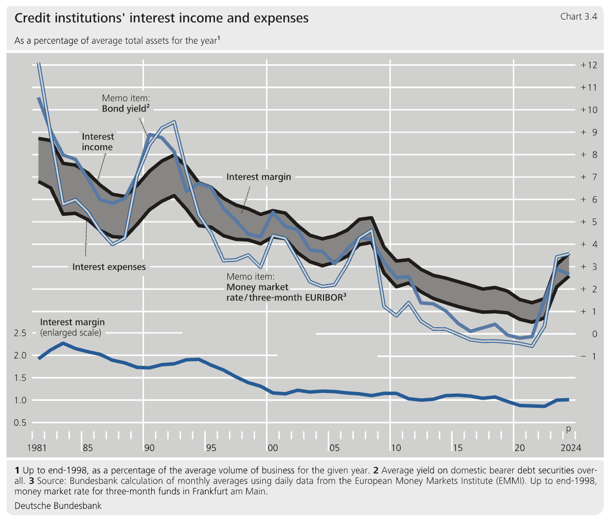
Aggregate data place individual institutions in context. The Bundesbank's historical interest series shows the long decline in nominal rates and gross interest flows, followed by the sharp repricing around 2022–2024. Interest income and expense move together over long periods, but not at the same speed. Their difference, expressed relative to the specified average asset base, is much smaller than either gross flow. The chart's historical note matters because the denominator used before 1999 is not identical to the later average-total-assets definition.
The 2024 income composition below shows that net interest income contributed 64.9% of operating income for all categories of German banks, net commission income 24.8%, trading income 7.1% and other operating results 3.2%. Savings banks and credit cooperatives depended more heavily on net interest income than big banks, which had larger fee and trading contributions. A category can exceed 100% for one revenue component when another component is negative; the percentages are a reconciliation of signed flows, not shares of positive revenues alone.
| Item | All banks | Big banks | Regional/other commercial | Landesbanken | Savings banks | Credit cooperatives | Mortgage banks | Building and loan associations | Special/central-support banks |
|---|---|---|---|---|---|---|---|---|---|
| Net interest income | 64.9 | 51.0 | 55.4 | 69.2 | 72.3 | 72.9 | 102.0 | 99.1 | 69.5 |
| Net commission income | 24.8 | 34.6 | 23.5 | 14.0 | 26.0 | 23.4 | -3.3 | -5.5 | 23.0 |
| Trading-portfolio result | 7.1 | 17.8 | 13.0 | 8.6 | 0.0 | 0.0 | 0.0 | 0.0 | 1.2 |
| Other operating result | 3.2 | -3.5 | 8.1 | 8.3 | 1.7 | 3.7 | 1.3 | 6.5 | 6.4 |
| Operating income | 100.0 | 100.0 | 100.0 | 100.0 | 100.0 | 100.0 | 100.0 | 100.0 | 100.0 |
| General administrative spending | -59.6 | -71.5 | -54.3 | -54.1 | -56.8 | -60.6 | -41.4 | -70.4 | -56.7 |
| Of which: staff costs | -30.2 | -30.9 | -25.1 | -27.2 | -34.0 | -33.6 | -19.5 | -27.4 | -28.9 |
| Of which: other administrative spending | -29.4 | -40.6 | -29.2 | -26.9 | -22.8 | -27.0 | -21.9 | -43.1 | -27.8 |
| Result from valuation of assets | -8.0 | -9.1 | -7.2 | -16.0 | -5.9 | -7.8 | -8.2 | -3.2 | -7.9 |
| Other and extraordinary result | -1.4 | 6.9 | -9.1 | 2.9 | -0.6 | -0.6 | -19.2 | -9.5 | -6.9 |
“Result from the valuation of assets” is broader than a pure loan-default measure: its precise coverage follows the Bundesbank's accounting classification. Describing the entire 8.0% charge as realised loan losses would erase that distinction. Administrative costs also differ across business models, so a higher share need not prove worse operating efficiency without considering the services supplied and revenue mix.
| Category | 2020 | 2021 | 2022 | 2023 | 2024 |
|---|---|---|---|---|---|
| All categories of banks | 2.71 / 1.12 | 5.03 / 3.22 | 4.83 / 3.86 | 8.36 / 6.18 | 8.43 / 6.14 |
| Commercial banks | −1.56 / −2.95 | 2.65 / 1.41 | 6.05 / 5.97 | 9.16 / 7.02 | 10.00 / 7.18 |
| Of which: big banks | −7.08 / −8.22 | −2.26 / −2.13 | 9.12 / 12.29 | 12.12 / 11.91 | 11.81 / 9.26 |
| Of which: regional and other commercial banks | 4.10 / 2.46 | 6.00 / 3.81 | 4.27 / 2.25 | 7.49 / 4.15 | 9.06 / 6.02 |
| Landesbanken | 1.29 / 0.84 | 4.02 / 2.26 | 4.77 / 2.72 | 7.45 / 5.01 | 8.84 / 7.31 |
| Savings banks | 5.36 / 3.36 | 6.27 / 4.22 | 4.74 / 2.82 | 10.17 / 7.09 | 10.34 / 7.25 |
| Credit cooperatives | 7.31 / 4.98 | 8.37 / 6.19 | 4.59 / 3.46 | 8.92 / 6.47 | 7.92 / 5.53 |
| Mortgage banks | 8.06 / 1.40 | 16.91 / 5.73 | 5.99 / 3.76 | 8.89 / 5.69 | 7.95 / 4.47 |
| Building and loan associations | 1.66 / 0.86 | 1.41 / 0.50 | 2.79 / 1.65 | 4.14 / 1.99 | 3.60 / 3.17 |
The return-on-equity series reports pretax values with after-tax values separately identified. For all categories, pretax ROE rises from 4.83% in 2022 to 8.36% in 2023 and 8.43% in 2024; the corresponding after-tax values are 3.86%, 6.18% and 6.14%. This improvement is consistent with a period in which asset income benefited from rising rates before all funding costs caught up. It does not imply that every institution benefited or that the same margin persists after deposit repricing and borrower stress. These ratios use annual average equity as defined in the statistical series, including the fund for general banking risks, rather than the year-end denominator of the earlier simplified example.
Historical aggregate data: Deutsche Bundesbank, The performance of German credit institutions in 2024, September 2025. The tables retain the report's preliminary 2024 status and accounting definitions.
Valuation, policy uncertainty and the deposit franchise
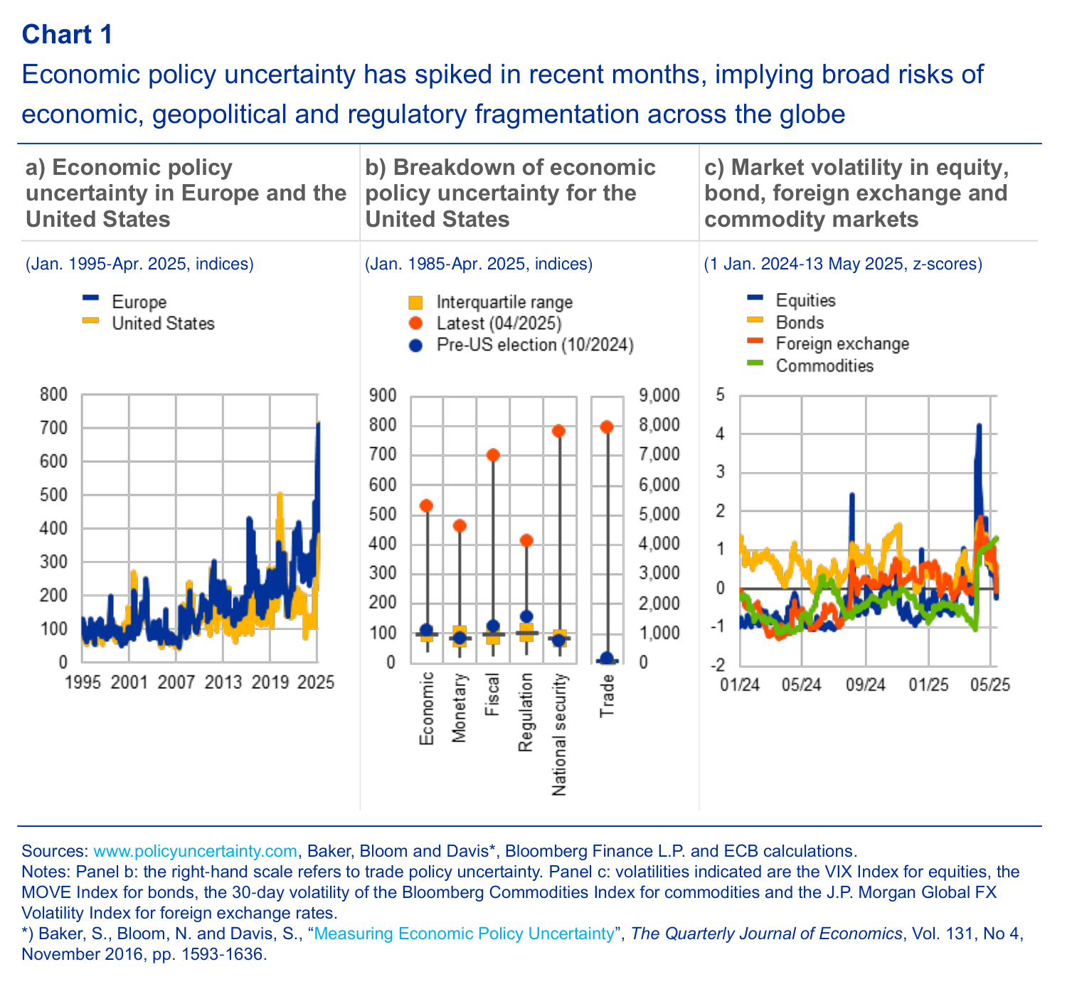
Market valuations add a forward-looking dimension to accounting performance. The ECB's May 2025 exhibits show a period of sharply elevated policy uncertainty alongside changing bank valuations and profitability. The uncertainty indices, market-volatility measures and bank price-to-book ratios have different units and should be interpreted separately. A high uncertainty reading is not itself a quantified bank loss; it indicates an environment in which investment decisions, funding conditions and asset prices may change abruptly.
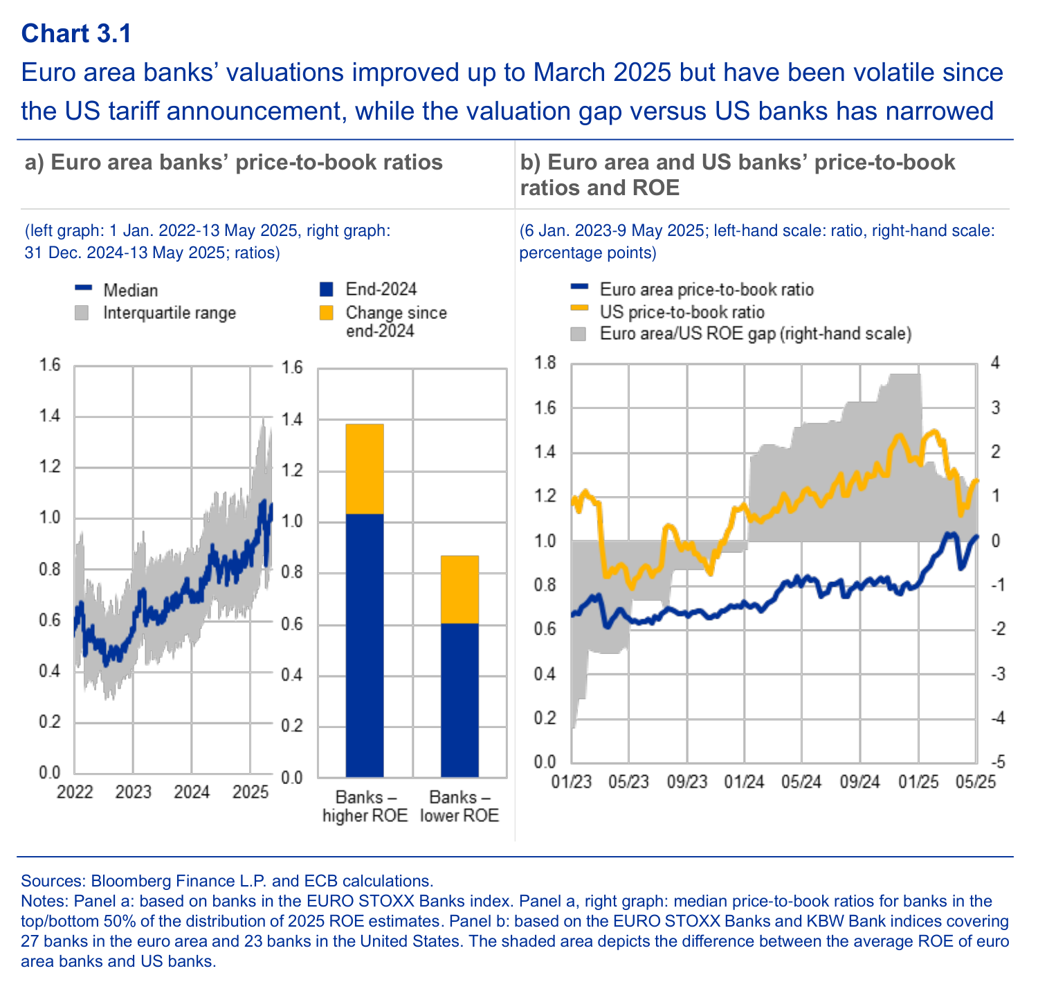
A price-to-book ratio compares the market value of equity with its accounting value. It can rise when investors expect more persistent earnings or require a lower risk premium; it can fall when they anticipate losses, dilution or poor future returns. A ratio below one does not by itself prove that a bank is insolvent. The ECB's 2025 comparison links valuation differences to profitability, but differences in business models, accounting and expected growth remain relevant when comparing the euro area with the United States.
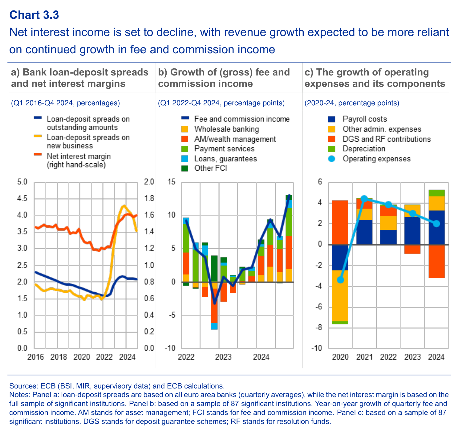
The profitability panels distinguish loan–deposit spreads, net interest margins, fee-income growth and changes in operating costs. A lender can experience a narrower new-business spread while its outstanding fixed-rate book reprices only gradually. An asset manager can earn more fees because client portfolios appreciate even without receiving new client money. Staff costs, deposit-guarantee contributions, resolution-fund contributions and depreciation can move differently. A credible earnings analysis therefore decomposes changes instead of attributing the whole profit movement to one policy rate.
The deposit franchise is the economic value of a bank's ability to maintain customer funding on favourable terms after paying the costs of providing account services. Customers value payment access, convenience, safety and an established relationship, so deposit remuneration need not immediately equal a wholesale market rate. When market rates rise faster than deposit rates, the funding advantage can increase. Competition, customers moving to term deposits, online comparison tools and withdrawals can later erode it. Maintaining the franchise also requires spending on technology, branches, service and compliance.
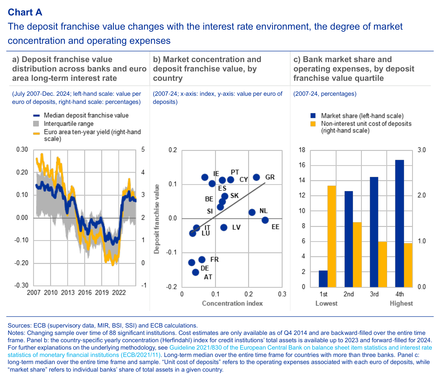
A constructed present-value expression makes the mechanism explicit. Let be expected deposits, the cost of comparable alternative funding, the deposit rate, the costs attributable to serving those deposits and an appropriate discount rate. Then a simplified franchise value is
This is a valuation framework rather than a measured number for a specific bank. It depends on deposit persistence, pricing, costs and risk. A large balance of expensive or unstable deposits can be less valuable than a smaller stable customer base. The franchise value is also not a stock of immediately available cash: relying on it to cover today's withdrawals would confuse expected future earnings with liquidity.
Historical European context: European Central Bank, Financial Stability Review, May 2025, including its analysis of deposit-franchise value. Accounting context for expected losses: BIS Financial Stability Institute, IFRS 9 and expected loss provisioning.
Financial statements are therefore a starting point for judgement. A robust assessment connects the asset mix, funding structure, income sources, loss recognition and available liquidity. Profitability that comes from an efficient service is economically different from profitability achieved by reducing capital, accepting illiquidity or increasing unrecognised risk. The numerical examples establish a discipline that applies throughout banking: state the denominator, specify the shock, reconcile the arithmetic and explain what the result does and does not measure.
3. Bank Lending: Contracts, Credit Analysis and Collateral
A bank loan combines a transfer of purchasing power today with a claim on future payments and a set of rights that govern what happens between those dates. Its value depends on the borrower's cash flows, but also on information, incentives, priority and enforcement. Good lending therefore involves much more than checking whether a borrower owns valuable assets: the bank must understand how the debt will be repaid, how repayment prospects could deteriorate, and what the contract allows it to do when they do.
Loans in the bank's asset portfolio
Lending is the largest asset category in the euro-area banking aggregates below. Its importance does not mean that every loan finances a household purchase or a business investment. Interbank claims and deposits held at the central bank are included in the loan statistics, so changes in aggregate loans can reflect liquidity management and monetary operations as well as credit supplied to the non-financial economy. Securities, meanwhile, include instruments that may expose the bank to credit and interest-rate risks similar to those arising from a loan.
| Asset category | 2000 | 2005 | 2010 | 2020 | June 2025 |
|---|---|---|---|---|---|
| Loans | 63% | 58% | 55% | 61% | 59% |
| Securities | 14% | 15% | 15% | 11% | 12% |
| Other assets | 24% | 27% | 29% | 28% | 29% |
| Total assets (EUR billion) | 16,662 | 23,635 | 32,207 | 35,930 | 41,383 |
| Borrower or loan category | 2000 | 2005 | 2010 | 2020 | June 2025 |
|---|---|---|---|---|---|
| Interbank, including central-bank deposits | 34% | 33% | 31% | 40% | 40% |
| Government | 8% | 6% | 7% | 5% | 4% |
| Corporates | 26% | 25% | 26% | 22% | 21% |
| Retail mortgages | 18% | 21% | 21% | 21% | 22% |
| Other retail | 11% | 9% | 8% | 6% | 6% |
| Other loans | 4% | 5% | 7% | 6% | 7% |
| Total loans (EUR billion) | 10,421 | 13,678 | 17,762 | 21,977 | 24,481.5 |
The percentages are rounded and need not sum to exactly 100%; neither should rounded asset shares be multiplied by totals to manufacture more precise loan amounts. Between 2000 and June 2025, the displayed stock of total assets increased substantially, while loans remained close to three-fifths of the balance sheet. Corporate lending and mortgages are large exposures, but interbank claims are sufficiently important that a bank's funding and counterparty network cannot be ignored in credit analysis.
Data: European Central Bank, aggregated balance sheet of euro-area monetary financial institutions, historical observations through June 2025. These are dated observations, not a statement of the latest balance-sheet position.
Term loans, revolving facilities and letters of credit
From the lender's perspective, granting a loan means acquiring a financial asset: an enforceable claim against the borrower's future cash flows. The principal advanced is the initial investment in that claim. Bank loans are often customised and relatively illiquid because outsiders do not possess all the information collected during negotiation and monitoring. A loan is an asset for the bank and a liability for the borrower; these two perspectives must not be confused when discussing interest income, funding costs or balance-sheet expansion.
A term loan supplies funds for a defined maturity, often to finance a fixed investment or refinance existing debt. A simple term loan is paid out in full at origination. An amortising structure repays principal gradually; a bullet structure leaves principal until maturity. A revolving credit facility instead permits borrowing, repayment and reborrowing during an availability period up to a contractual limit. The undrawn commitment matters because the bank may need to provide cash exactly when the borrower becomes more dependent on it. Interest on amounts drawn and a commitment fee on undrawn amounts perform different economic functions.
A letter of credit is a bank undertaking to pay a beneficiary when specified documentary conditions are satisfied, widely used in trade. It resembles a guarantee in providing the bank's credit standing, but a documentary credit and a standby guarantee need not have the same payment conditions. Its initial exposure may be contingent rather than a cash loan. If the bank pays and the customer does not immediately reimburse it, the contingent commitment becomes a funded credit exposure.
The distinction between loans and bonds is a matter of degree. Both are debt claims, and both can be secured, floating-rate or covenant-protected. Bonds are usually more standardised and easier to trade; loans often involve private information and active monitoring. Loan sales and securitisation can transfer a loan's economic risk beyond the originating bank, so the institution that originates, funds, services and ultimately bears the risk need not be the same.
The lending process and its information problems
Origination begins with identifying a customer's financing need, receiving an application, assessing creditworthiness and negotiating a contract, including its price. Funding then supplies the agreed resources once the relevant conditions are met. Servicing records balances, collects interest and principal, and administers contractual obligations. Risk processing continues after disbursement through monitoring, portfolio diversification, interest-rate management and, when necessary, restructuring or recovery. The bank's credit culture governs who can approve a loan, how exceptions are reported and whether staff are rewarded for sound long-term repayment or simply for lending volume.
| Function | Main task | Reason it matters |
|---|---|---|
| Origination | Application, screening, contract design and pricing | Select viable borrowers and establish terms before exposure arises |
| Funding | Provide funds after approval and fulfilment of drawdown conditions | Convert a commitment into a funded asset without losing liquidity control |
| Servicing | Bookkeeping and collection of contractual payments | Maintain reliable balances and identify arrears promptly |
| Risk processing | Monitoring, diversification, workouts and interest-rate risk management | Control losses and exposures throughout the life of the claim |
| Credit culture | Organisation, reporting, communication and staff incentives | Make individual decisions consistent with the bank's risk capacity |
Adverse selection concerns information hidden before contracting: applicants know more about their ability or intentions than the bank does. Screening and credit analysis try to distinguish these types. Moral hazard concerns actions taken after financing: the borrower may substitute a riskier project, reduce effort, divert assets or prioritise other creditors. Contract design and monitoring seek to influence those actions. A favourable initial credit score cannot prevent an owner from changing business strategy after the loan has been paid out.
Two forms of moral hazard are especially useful to distinguish. Asset substitution increases project risk after the lender has fixed its promised return; limited liability allows shareholders to capture part of the upside while creditors bear more downside. Effort aversion arises when the borrower bears the private cost of careful management but shares the resulting improvement in repayment prospects with the lender. Capital at risk, collateral, covenants and the prospect of future borrowing can all alter these incentives, though none eliminates the need to assess project viability.
Financial terms, covenants and control rights
A loan contract specifies principal, interest, fees, drawdown conditions and repayment dates. A floating interest rate changes with a benchmark plus an agreed margin; a fixed rate remains constant over its specified period. Floating rates reduce some interest-rate mismatch for the lender, but may increase borrower default risk when debt service rises. Fees also matter: an up-front facility fee or a recurring commitment fee means that the borrower's financing cost is not captured by the stated coupon alone.
Representations and warranties establish facts asserted at contracting, such as the accuracy of financial statements, authority to borrow, title to assets and disclosed litigation. Affirmative covenants require continuing actions, including reporting, maintaining insurance and paying taxes. Negative covenants restrict conduct, such as asset sales, additional liens, mergers or dividends. Financial covenants impose measurable thresholds, for example a maximum debt-to-EBITDA ratio or a minimum interest-coverage ratio. A financial covenant is often economically restrictive even if the agreement places it under an affirmative-covenant heading.
These provisions transfer control rights before a borrower necessarily misses a payment. A covenant breach can lead to a waiver, additional reporting, revised pricing, more security or acceleration if the contract and applicable law allow it. The existence of a breach does not mean that immediate liquidation is always the bank's best response. It can be more valuable to renegotiate a viable business than to enforce against assets at distressed prices. Covenant definitions must therefore be read carefully: permitted EBITDA adjustments, accounting conventions, testing dates and cure provisions can materially change the same apparently simple ratio.
| Family | Provision | Investment grade (n = 3,533) | Non-investment grade (n = 945) | Total (n = 4,478) |
|---|---|---|---|---|
| Investment restrictions | Indirect investment restrictions | 7.8 | 42.43 | 15.1 |
| Investment restrictions | Merger restrictions | 91.8 | 93.3 | 92.1 |
| Investment restrictions | Secured | 3.0 | 5.3 | 3.5 |
| Investment restrictions | Stock sale restrictions | 1.5 | 3.7 | 2.0 |
| Investment restrictions | Direct investment restrictions | 0.04 | 2.4 | 0.8 |
| Investment restrictions | Any investment restriction | 93.8 | 94.3 | 93.9 |
| Dividend restrictions | Dividend payment restrictions | 5.5 | 39.0 | 12.6 |
| Dividend restrictions | Restrictions on other payments | 5.0 | 43.0 | 13.1 |
| Dividend restrictions | Dividend or other payment restrictions | 6.2 | 44.0 | 14.2 |
| Subsequent financing | Subordinate debt issuance | 74.1 | 66.6 | 72.5 |
| Subsequent financing | Sale and lease obligations | 58.1 | 40.3 | 54.3 |
| Subsequent financing | Debt priority | 15.8 | 49.5 | 22.9 |
| Subsequent financing | Stock issuance | 5.1 | 28.1 | 10.0 |
| Subsequent financing | Any subsequent financing restriction | 78.4 | 73.2 | 77.3 |
| Event restrictions | Default-related event covenants | 51.7 | 71.0 | 55.8 |
| Event restrictions | Change-of-control poison put | 24.4 | 74.2 | 34.9 |
| Event restrictions | Any event restriction | 60.0 | 88.7 | 66.1 |
The bond sample covers US-domiciled non-financial issuers over 1993–2007. The categories overlap: a bond can restrict dividends and borrowing at the same time, and a family total is not the sum of all its rows. The sharp difference in dividend and change-of-control provisions illustrates how contracts respond to conflicts between shareholders and creditors. It does not imply that every covenant is more common in speculative-grade bonds; the table contains counterexamples.
| Covenant | Loans | Loan packages | Mean amount (USD bn) | Median amount (USD bn) | Total amount (USD bn) |
|---|---|---|---|---|---|
| Maximum debt to EBITDA | 7,544 | 4,417 | 0.20 | 0.09 | 1,480.53 |
| Minimum tangible net worth | 7,196 | 4,931 | 0.13 | 0.03 | 926.67 |
| Minimum fixed-charge coverage | 6,064 | 3,514 | 0.14 | 0.06 | 842.95 |
| Minimum interest coverage | 5,856 | 3,486 | 0.22 | 0.10 | 1,299.70 |
| Maximum leverage ratio | 2,401 | 1,748 | 0.32 | 0.15 | 758.06 |
| Maximum debt to tangible net worth | 2,331 | 1,677 | 0.06 | 0.01 | 137.90 |
| Minimum current ratio | 2,098 | 1,455 | 0.06 | 0.02 | 126.45 |
| Minimum debt-service coverage | 1,906 | 1,186 | 0.07 | 0.01 | 126.08 |
| Maximum senior debt to EBITDA | 1,654 | 857 | 0.14 | 0.09 | 231.34 |
| Minimum EBITDA | 1,556 | 886 | 0.09 | 0.04 | 135.32 |
| Minimum quick ratio | 779 | 555 | 0.02 | 0.01 | 19.16 |
| Minimum cash interest coverage | 321 | 165 | 0.19 | 0.10 | 60.70 |
| Maximum debt to equity | 169 | 119 | 0.17 | 0.04 | 27.95 |
| Maximum senior leverage | 20 | 10 | 0.23 | 0.12 | 4.54 |
| Maximum loan to value | 19 | 8 | 0.05 | 0.02 | 0.97 |
A loan package can contain several facilities, which explains why the number of loans exceeds the number of packages. The amount columns describe the loans associated with each covenant, not the covenant thresholds. For instance, 0.20 billion in the first row is an average loan amount, not a debt-to-EBITDA limit. A single loan can appear under several covenants, so adding the monetary totals across rows would double-count exposures.
Historical covenant tables: Chava, Fang, Kumar and Prabhat (2019), Debt Covenants and Corporate Governance, reviewing the bond evidence of Chava, Kumar and Warga (2010) and the loan evidence of Chava and Roberts (2008). The loan data combine non-financial-firm records from CRSP/Compustat and DealScan; EBITDA means earnings before interest, taxes, depreciation and amortisation.
A real loan agreement: the North Wabash residential financing
The 9 November 2012 residential term-loan agreement between 401 North Wabash Venture LLC, as borrower, and Deutsche Bank Trust Company Americas, as lender, shows how these mechanisms fit together. Its stated maximum principal was USD 53,730,977.65, to be advanced in full at closing. The proceeds refinanced existing debt secured on the mortgaged premises and associated customary closing costs. Principal repaid could not be borrowed again: this was a term loan, not a revolver. The residential facility must also be distinguished from the separate commercial loan to which several provisions referred.
The agreement identified Donald J. Trump as guarantor and Trump Chicago Residential Manager LLC as the manager. Their economic roles differ: the borrower owes the loan, the guarantor supports specified obligations, and the manager operates the relevant property. This is a historical contract study; its rates, dates, thresholds and remedies are the negotiated 2012 terms, not current standard conditions for every property loan.
| Term | Contractual provision | Economic purpose |
|---|---|---|
| Principal and availability | USD 53,730,977.65, fully funded at closing; no reborrowing | Refinancing rather than a continuing working-capital commitment |
| LIBOR option | Relevant USD LIBOR plus 3.35 percentage points annually | Benchmark compensation plus borrower-specific margin |
| Ordinary prime option | Prime rate plus 1.00 percentage point annually | Alternative floating-rate convention |
| LIBOR-failure fallback | Conversion at prime minus 0.50 percentage points under section 2.2(b) | A distinct contingency rule, not the ordinary prime-option margin |
| Interest computation | Actual days/360 for LIBOR; actual days/365 for prime | Day-count conventions affect the cash interest paid |
| Facility fee | 0.625% of initial loan, payable at closing | Up-front compensation of approximately USD 335,818.61 |
| Original maturity | 8 November 2016, unless accelerated or validly extended | Defines the refinancing and final repayment deadline |
| Conditional extension | To 7 November 2017; principal no more than USD 6 million, LTV no more than 25%, no specified continuing defaults and required fees paid | Extension depends on deleveraging and collateral protection |
| Extension fee | 0.25% of outstanding principal | USD 15,000 if principal is exactly USD 6 million |
| Default interest | Greater of prime + 4 percentage points or the otherwise applicable loan rate + 4 percentage points, capped at the maximum permitted rate | Applies during a continuing event of default and replaces ordinary interest |
| Late charge | 5% of overdue amounts after applicable notice/cure periods, subject to contractual and legal limitations | Compensation for handling delinquency, distinct from default interest |
LIBOR interest periods could be 30, 90 or 180 days, or 12 months, subject to the agreement. Interest was payable at the end of the period and, for periods longer than 90 days, also at three-month intervals. Prime-rate interest was payable monthly. The contract limited simultaneous LIBOR advances to five, with at least USD 1 million in each separately selected period. If a swap was chosen, its index and the loan's interest-period election had to be coordinated. A swap was optional, but obligations under it could receive security and guarantee protection under the loan documents.
For an illustrative, unchanged USD 10 million balance at a 4% annual LIBOR-based contractual rate over 90 actual days, the interest is dollars. A 365-day denominator would produce approximately USD 98,630.14 for the same numerical rate and days. The example isolates the day-count effect; it is not a reconstruction of actual payments. LIBOR has since ceased publication, so studying the old clause does not imply that a new loan should use it.
Historical contractual terms: Term Loan Agreement (Residential), 9 November 2012, sections 1.1 and 2.1–2.18. For the subsequent benchmark transition, the Financial Conduct Authority records that the final remaining synthetic LIBOR settings were published on 30 September 2024.
Repayment, property sales and collateral control
The North Wabash loan combined a final maturity with mandatory reductions in principal. Sales of residential units, parking units and storage units generated release payments to the bank. A unit could be released from the mortgage only under the agreed closing and documentation conditions, including receipt of the required payment and the absence of a disqualifying default. The lender therefore did not simply rely on the borrower promising to use sale proceeds responsibly: release of collateral was tied to reduction of its exposure.
| Anniversary of closing | Minimum principal repaid cumulatively (USD) | Initial principal less this cumulative amount (USD) |
|---|---|---|
| First | 11,932,744.41 | 41,798,233.24 |
| Second | 23,865,488.83 | 29,865,488.82 |
| Third | 35,798,233.24 | 17,932,744.41 |
| Fourth | 47,730,977.65 | 6,000,000.00 |
The repayment column is cumulative: the second-anniversary amount already includes the first-anniversary requirement. Excess repayments counted toward subsequent minimums. If sales and other repayments fell short, the borrower or guarantor had to provide the difference from other resources. The USD 6 million balance in the last row is not an unconditional right to leave that amount outstanding beyond the original maturity; without a valid extension, all remaining principal was due at maturity.
The release payment for a unit was the greater of its scheduled minimum release price and its required release price. The latter broadly meant the adjusted gross sales proceeds less permitted selling costs and reimbursable furniture, fixtures and equipment costs for eligible model units. The specified category of customary closing costs, commissions and related deductions was capped at 8% of the gross sales price. Thus a nominal sale price alone does not reveal the amount left for the borrower. The minimum release schedule prevents an unusually low sale price from eroding the lender's remaining collateral cushion without an adequate paydown.
Voluntary prepayments generally required three business days' notice and at least USD 1 million, with USD 100,000 increments above that amount, unless paying the smaller remaining balance in full. The agreement described prepayment as free of a premium or penalty, while still requiring specified LIBOR breakage and increased-cost compensation. Those are economically relevant potential costs: “no prepayment penalty” does not necessarily mean that every early repayment has zero cash consequence. Taxes, withholding gross-ups and changes in regulatory funding costs were also allocated by explicit clauses.
The residential collateral carried a first-priority security interest, subject to permitted encumbrances, and the demand deposit account was part of the collateral package. The residential facility additionally benefited from a second-priority claim on the commercial mortgaged premises, while the commercial facility benefited from cross-collateralisation in the other direction under its documents. These arrangements had defined termination conditions. Priority matters because a second lien only reaches value remaining after the prior claim; saying that two loans are secured by the same building does not mean that their recoveries are identical.
Section 2.10 also provided for an unconditional guarantee of outstanding principal and interest, together with operating shortfalls during the contractually defined coverage period. Its reference to a separate guaranty matters: the loan agreement describes that support, but all detailed limits and mechanics must be read with the actual guaranty rather than invented from a property valuation. A guarantee is a claim on a person; collateral is a claim against identified assets. Their value depends on different recovery channels and can be correlated when guarantor wealth falls with the property market.
Covenants, default and the supporting documents
The historical LTV covenant limited outstanding debt to 57% of appraised mortgaged-property value before the original maturity and to 25% afterward. After the second anniversary, the lender could obtain an appraisal at its own expense to test the ratio. A shortfall could be addressed with a principal paydown, eligible cash or cash-equivalent collateral, or a combination. For this calculation, additional LTV collateral was deducted from the loan numerator rather than treated as another piece of property in the denominator.
With debt , eligible pledged cash and appraised property value , the adjusted test can therefore be expressed as , where is the applicable 0.57 or 0.25 limit. An illustrative debt balance of USD 30 million against USD 50 million of property is at 60% LTV. To reach 57%, the borrower must reduce the adjusted debt by million dollars. The example is a calculation of the contract's mechanism, not a claim about the property's actual historical valuation.
The agreement included notice and appraisal-dispute procedures. Before treating an apparent shortfall as an immediately enforceable default, the bank had to consider the relevant cure and dispute provisions, including the mechanism for an independent third appraisal. A drafting inconsistency in one extension passage used the words “twenty percent” beside “25%”; the repeated substantive extension and covenant provisions specify 25%. This is precisely why a contractual analysis should reconcile the operative clauses rather than copy an isolated phrase.
Information rights required annual financial statements and a compliance certificate within 120 days of calendar-year end, and quarterly sales and unit-closing reports within 45 days of quarter-end. The annual financial statements were specified as unaudited, prepared by independent certified public accountants and certified by a responsible borrower officer; describing them simply as audited accounts would be incorrect. The agreement also required access to records and information about relevant defaults, material changes, taxes and condominium operations.
Other affirmative obligations maintained insurance, property condition, legal permissions, environmental compliance and separate-entity status. Negative covenants restricted new liens, transfers, mergers, additional debt, affiliate transactions and loans to others. Distributions were prohibited while an event of default continued. The special-purpose-entity provisions, management arrangements and insurance obligations all protect the value that ultimately supports repayment; they are economically connected to credit risk even when they do not look like an interest-rate clause.
Events of default extended beyond missed principal. They included unpaid interest or fees after the specified three-business-day period, material misrepresentation, defined covenant failures, relevant insolvency proceedings, loss of security, prohibited assignments, change of control and specified management misconduct. The cross-default provisions linked this loan to other debt, including a threshold above USD 20 million for debt to outside creditors, subject to the detailed acceleration, contest and collateral conditions. Material judgments above USD 10 million were separately addressed. Some breaches had cure periods, some could be accelerated automatically, and some allowed the lender to choose acceleration. None of these distinctions can be collapsed into “any problem makes the loan immediately due.”
On a continuing default, contractual remedies included acceleration, use of cash collateral, foreclosure and exercising specified rights over contracts and receipts. The lender could act as attorney-in-fact for defined protective purposes; this did not make it a partner in the project. This was a bilateral lender-borrower agreement, not evidence of a separate syndicated-loan administrative agent. It allowed assignments and participations under specified consent and counterparty conditions. With a participation, the original lender remained the holder of the agreement and note and the borrower continued dealing directly with it, illustrating how funding or risk can be shared without replacing the borrower's operational counterparty.
The supporting schedules turn broad promises into verifiable procedures. Sales-contract forms cover residential units, parking and storage; the minimum-release-price schedule identifies individual collateral items; the promissory note records indebtedness; conversion notices select interest options; and release forms document removal of a lien. Organisational charts identify ownership and control. The management agreement, service-contract exceptions and the manager's consent address operating continuity, fees, reporting, termination and lender recognition. A compliance-certificate form makes recurring monitoring concrete. The loan agreement generally chose New York law while reserving creation, perfection and enforcement of property liens to the law of the property's location. Conditions precedent required the documentary and due-diligence package to be in place before funding, including executed loan documents, title and security evidence, property and environmental reports, insurance, fees and the related commercial-loan documents. These closing conditions reduce the risk that funds are advanced before promised protections actually exist. These documents are part of the credit design, but individual unit inventories, blank signature blocks and repeated legal forms do not need to be reproduced to understand the lending mechanism.
Creditworthiness through the five Cs
The five Cs organise evidence rather than replace judgement. Capacity asks whether the borrower has both the legal authority to borrow and the economic resources to pay. Corporate assessment connects liquidity, inventory and receivables turnover, profitability, leverage and forward-looking cash flows. Household assessment compares sustainable verified income with expenditure, existing debts and possible changes in interest costs or employment. The analyst should reconcile accounting profit with cash available for debt service: an apparently profitable firm can still be unable to repay because customers have not paid or a large bullet maturity is approaching.
A useful measure is the debt-service-coverage ratio:
Both quantities must cover the same period and follow a defined convention for taxes, working capital, maintenance investment and other commitments. Cash flow of EUR 1.2 million against scheduled debt service of EUR 1 million gives . The EUR 0.2 million cushion may be eroded by a sales decline or unexpected maintenance cost. A ratio above one in the base case therefore does not make stress analysis unnecessary.
Character concerns the willingness to honour obligations, inferred from repayment behaviour, the reliability of information and prior dealings. Credit-bureau records, commercial information providers and the bank's own account history provide different types of evidence. Examples include Creditreform and Dun & Bradstreet for firms and SCHUFA or US consumer credit-bureau reports and FICO scores for households. A bureau and a scoring model are not the same institution or product: the score summarises selected information, whereas the underlying report contains the credit history used to construct it.
Capital means the owner's funds or wealth at risk. It absorbs part of the downside and can signal confidence in the project. Collateral identifies assets the lender may recover under the security arrangement. Inside collateral belongs to the financed business; outside collateral is additional wealth, such as an entrepreneur's personal house. Conditions cover industry competition, customer concentration, supplier dependence, legislation, the business cycle, household job security and the housing market. Weak conditions can reduce both operating cash flow and collateral value at the same time.
| Information source | What it can reveal | Main limitation |
|---|---|---|
| External credit information | Existing obligations, arrears and prior repayment behaviour | Coverage, errors, timing and differing score definitions |
| Relevant applicant and employment characteristics | Income stability and economic circumstances | Predictive association alone does not establish permissible or fair use |
| Income, expenditure, assets and liabilities | Capacity and affordability | Self-reported figures may need verification and stress testing |
| Previous loan performance | Observed willingness and ability to repay | A new customer may have no history with the lender |
| Current-account behaviour | Overdrafts and variability of receipts or spending | Available chiefly to an incumbent bank and subject to data-use constraints |
| Expert review and a second-person check | Context not captured by a mechanical score | Judgement can be inconsistent or biased without documented controls |
Historical retail scorecards also used demographic categories such as age, gender, marital status and occupation. Describing those inputs does not endorse their use: a variable's predictive association and its legal or fair use are separate questions. Some digital lenders also analyse an applicant's digital footprint. More data do not automatically produce a better or acceptable lending decision: data quality, explainability, privacy and discriminatory effects require attention. Historical lists of demographic variables used in scoring describe past practices, not permission to use every such characteristic in a present-day credit model. The incumbent bank's information advantage arises especially from previous loans and account transactions, which competitors may be unable to observe.
For the governance and lifecycle assessment of lending, see the European Banking Authority's Guidelines on loan origination and monitoring. Creditworthiness must be assessed alongside the valuation and monitoring of collateral.
Collateral as recovery, incentive and signal
Collateral has three distinct functions. First, enforceable recovery reduces the lender's loss if default occurs. Second, the prospect of losing pledged assets can encourage effort and repayment after contracting. Third, willingness to pledge assets can reveal information before the bank grants the loan. An observed secured loan can involve all three, but a given example may be driven mainly by one. Collateral can sometimes make a positive-net-present-value investment financeable by reducing agency costs or assigning a new lender a credible recovery claim. This can reduce underinvestment, meaning that a socially or jointly valuable project is not undertaken because the borrower cannot obtain funds or capture enough of its benefit. It does not eliminate every debt-overhang problem, in which existing creditors capture much of the benefit of a new investment. A wealthy borrower with poor prospects can still post security, and a capable but asset-poor borrower may be unable to do so, so collateral is not an infallible signal.
Consider three cases. A government pledges an aircraft but avoids foreign trips after default so that creditors cannot seize it: even if recovery never occurs, the lost use of the aircraft can impose a cost on non-payment, illustrating an incentive effect. A transparent company grants a new bank a first claim on plant and equipment: the central effect is improved priority and recovery relative to other lenders. An opaque entrepreneur is asked to pledge a private home: the willingness to expose personal wealth may help screen project quality before lending.

The historical Argentine aircraft report illustrates how the threat of attachment abroad can change behaviour even when a creditor never obtains the asset. The news episode should not be mistaken for proof that the aircraft had been voluntarily pledged under a particular loan contract. The stylised collateral example isolates the incentive mechanism; the article illustrates the broader role of enforcement risk in a sovereign debtor's decisions.
A familiar early-FedEx anecdote attributed to manager Roger Frock describes Fred Smith risking the company's last USD 5,000 at blackjack when an approximately USD 24,000 fuel bill threatened operations, then returning with USD 27,000. Treated as an anecdote rather than a recommended financing strategy, it illustrates gambling for survival: when ordinary continuation appears impossible, the decision-maker may prefer a small chance of rescue to certain failure. A successful realised gamble does not establish that its expected value was positive or that it protected creditors.
A different historical account concerns the 1990 restructuring of Trump-related businesses. The account describes more than USD 2 billion of debt, a missed USD 30 million interest payment, negotiations with major banks alongside many smaller creditors and secured bondholders, an additional USD 65 million of financing, and deferred interest on about USD 850 million of bank loans. Its economic lesson is creditor coordination: one creditor's enforcement can destroy going-concern value for others, while new financing may preserve that value if the underlying business remains viable. Forbearance is therefore not automatically irrational, but neither does it prove solvency; lenders must distinguish a credible restructuring from postponing recognition of losses.
The aircraft clipping is an NPR report dated 10 January 2013. The FedEx story is a reported management recollection; the 1990 restructuring account follows the historical account attributed to Horowitz and Goodwin (1990). These examples illustrate incentives and coordination rather than establish general causal estimates.
Recovery values and expected credit loss
Nominal collateral value is not the amount a creditor necessarily receives. Prior liens, legal costs, delays, deterioration and the discount required for a forced sale all matter. If is exposure at default and is the present value of proceeds available to this lender after costs, a simplified loss fraction is:
Here is loss given default, measured conditional on default; the formula needs adjustment to the selected accounting or regulatory methodology where applicable. For a EUR 500,000 exposure and recoveries of EUR 300,000, the loss is EUR 200,000 and . With a one-year default probability , expected credit loss is euros. If recoveries fall to EUR 150,000, rises to 70% and expected loss to EUR 10,500, although the assumed probability of default is unchanged.
This distinction separates frequency from severity. A recession can worsen both, especially when collateral is closely tied to the borrower's business. A EUR 4 million facility with and has euros over the specified horizon. Expected loss is a probability-weighted average, not a maximum possible loss, a capital requirement or an automatic accounting entry. Pricing, provisioning and capital models use related information for different purposes.
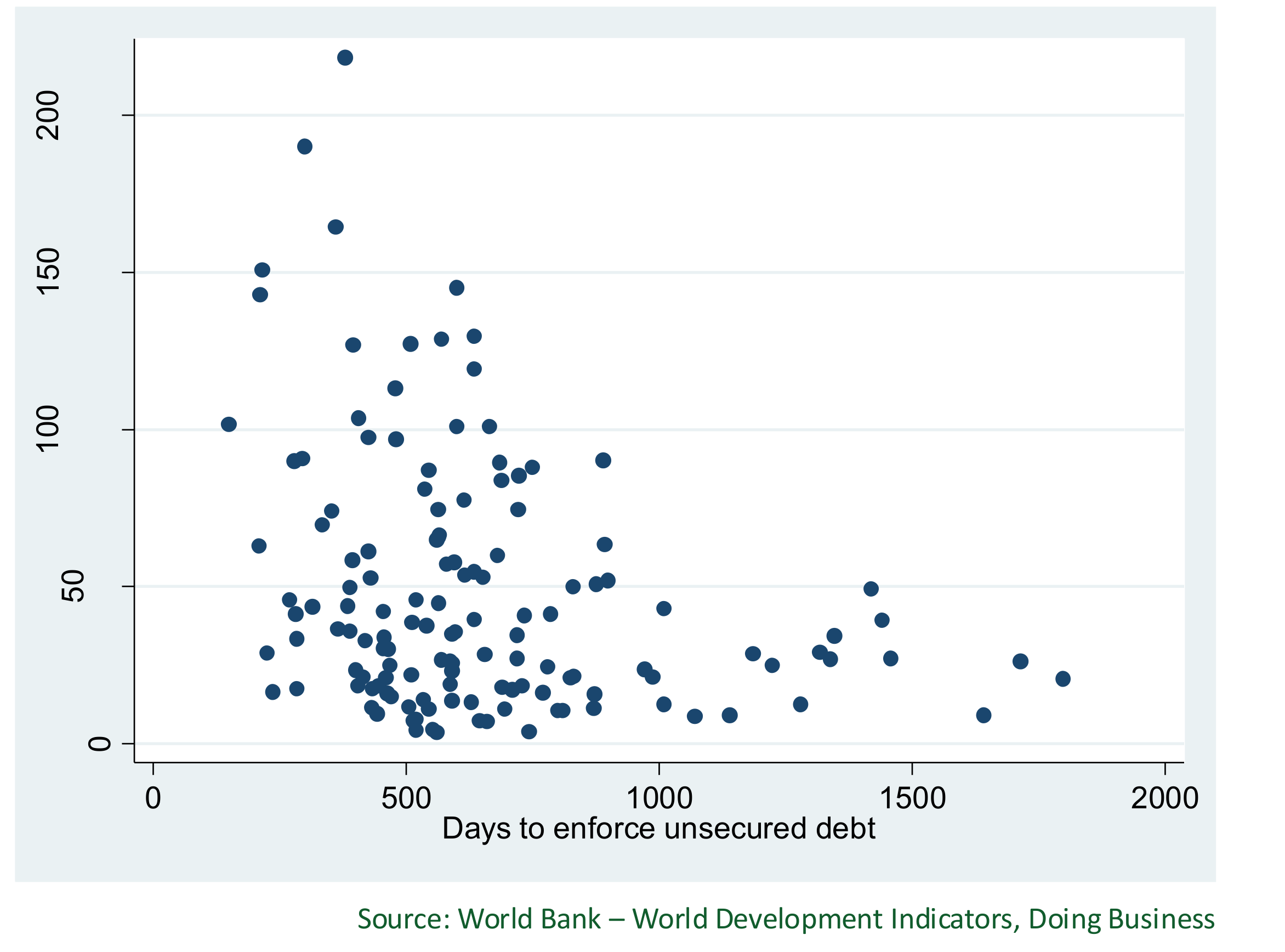
The historical scatter relates the time required to enforce unsecured debt to a credit-development indicator. Its pattern is consistent with slower enforcement being associated with less developed credit markets, but the supplied chart does not label the vertical measure precisely. It supports a qualitative illustration, not a numerical estimate of an effect or an assertion about a particular country's current credit-to-GDP ratio. Income, institutions and reverse causality could also contribute to the association. The contractual lesson remains that a claim's value depends on how and when it can be enforced.
A complete screening example with and without collateral
Two risk-neutral entrepreneurs each need EUR 100. The safe entrepreneur produces EUR 140 with certainty. The risky entrepreneur produces EUR 140 with probability one-half and EUR 50 with probability one-half. The bank cannot identify their types and initially lends to both in equal proportions. Funding costs are zero, there are no enforcement costs and borrowers have limited liability unless they explicitly pledge outside wealth. Let be the one-period interest rate and the promised repayment.
In the unsecured contract, the safe entrepreneur pays and the risky entrepreneur pays in the high state but only EUR 50 in the low state. Provided , the bank's break-even condition for the two loans is:
The safe entrepreneur receives euros with certainty. The risky entrepreneur receives EUR 23.3333 in the good state and zero in the bad state, giving an expected private surplus of EUR 11.6667. Both therefore borrow. Yet the risky project's expected output is only euros, below its EUR 100 resource cost. Limited liability makes the project privately attractive because some downside is shifted to the lender and, through pooled pricing, the safe borrower.
| Outcome | Safe borrower | Risky borrower |
|---|---|---|
| Expected project output | EUR 140 | EUR 95 |
| Project NPV at the zero discount rate | EUR 40 | −EUR 5 |
| Unsecured expected bank receipt at r = 16.6667% | EUR 116.6667 | EUR 83.3333 |
| Unsecured expected borrower surplus | EUR 23.3333 | EUR 11.6667 |
| Secured bank receipt at r = 0% if the contract is accepted | EUR 100 | EUR 100 in either state |
| Secured expected change in borrower wealth | EUR 40 | −EUR 5 |
| Decision under the secured contract | Borrow | Do not borrow |
Now suppose each entrepreneur owns a house worth EUR 80 that can be pledged and sold without cost. At a zero interest rate, even the risky entrepreneur's low project payoff of EUR 50 plus sufficient collateral covers the EUR 100 debt. A competitive break-even secured contract can therefore set . The safe borrower earns EUR 40 and never loses the house. In the risky low state, the bank takes EUR 50 from the house to cover the shortfall; the borrower retains the residual EUR 30 of house value. The entire EUR 80 pledge is not an up-front fee and should not be subtracted in both states.
The risky borrower's change in own wealth is EUR 40 in the high state and minus EUR 50 in the low state. Expected surplus is consequently euros, so this borrower rejects the secured contract. Collateral has screened out the negative-NPV project by making its owner internalise the downside. EUR 80 is sufficient, though EUR 50 of perfectly realisable collateral would already cover the worst repayment shortfall in this particular model.
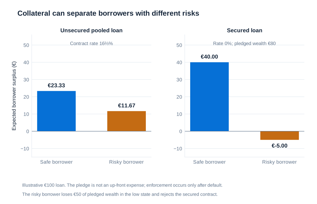
The model also reveals a distributional trade-off. If the safe entrepreneur lacks pledgeable wealth, an otherwise valuable project may fail to obtain the attractive secured contract. Requiring collateral can improve selection among equally wealthy applicants while excluding capable but poorer applicants. Neither “collateral is always efficient” nor “collateral is merely an unnecessary obstacle” follows from the example. The outcome depends on available information, wealth distribution, recoverability and alternative ways to screen borrowers.

Schmalz, Sraer and Thesmar's research on French administrative data uses changes in local house values to study this channel. Greater available housing collateral is associated with increased entry into entrepreneurship and, among entrants, greater debt use and larger firms. The study compares homeowners exposed to collateral gains with local groups that do not experience the same borrowing-capacity change, helping separate collateral from local demand. This empirical setting supports the relevance of pledgeable wealth; it does not turn the two-entrepreneur example into a universal prediction about every credit market.
Schmalz, Sraer and Thesmar, Housing Collateral and Entrepreneurship, Journal of Finance, 2017. The contract, recovery and screening examples together show why lending terms must be designed jointly with the information used to approve the loan.
4. Loan Pricing, Credit Rationing and Relationship Banking
A bank must earn enough on a loan to compensate for the resources used to originate and service it, the losses expected from default and the funding supplied by depositors and shareholders. However, a higher quoted interest rate is not always a route to a higher expected profit. The rate can change who applies and how a borrower behaves after receiving funds. This chapter connects a transparent pricing calculation to adverse selection, quantity rationing and the value of borrower-specific information.
The economic components of a lending rate
Let be the principal of a simple one-year loan, its operating cost in currency units, its probability of default, the fraction of exposure lost conditional on default, the fraction of funding allocated to equity, the cost of debt funding and the required return on equity. If exposure at default equals principal, a useful additive pricing benchmark is:
All rates and fractions in this equation use the same one-year horizon and are entered as decimals. Multiplication by 100 expresses the resulting rate as a percentage; one basis point is 0.01 percentage point, or 0.0001 in decimal form. The equation treats required annual interest revenue as the sum of operating cost, expected loss and a funding charge. It is a planning decomposition rather than a universal exact cash-flow valuation formula: fees, repayment timing, recoveries, defaulted interest, maturity and the treatment of capital can change the precise contractual rate.
Operating costs include screening the applicant, monitoring performance and collateral, servicing payments and allocated overhead such as systems, premises and management. Some are fixed per account rather than proportional to principal. A EUR 5,000 annual cost is 0.5% of a EUR 1 million loan but 5% of a EUR 100,000 loan. Scale can therefore influence pricing even when borrowers have the same default probability. Allocation also depends on loan type, operational efficiency and which services are shared across the customer relationship.
A break-even estimate answers whether the loan compensates the bank for its costs under stated assumptions. It does not tell the bank what rate it can actually charge. Competition, bargaining, switching costs, differentiated services and information determine the feasible margin. Cross-selling may justify assessing profitability across several services, but an anticipated fee from another product must be a credible economic benefit, not a device for concealing an underpriced loan.
Expected loss, exposure and the meaning of a rating
The basic expected-loss decomposition is:
is an expected monetary loss; is exposure at default; is a default probability for the selected horizon; and is the expected proportion lost after default, including the chosen treatment of recoveries and costs. For revolving commitments, can exceed the current drawn balance if the borrower draws more before failing. For long loans, a one-year PD must not be confused with the probability of ever defaulting over the full maturity. The decomposition also requires consistent assumptions about exposure and severity when these vary with economic conditions.
For euros, and , euros. This is an average over uncertain outcomes, not a prediction that each loan will lose exactly EUR 8,000. Unexpected losses around that average motivate capital and risk limits. An accounting loss allowance and a regulatory capital charge have different objectives and may use different horizons and model constraints, so neither should be equated mechanically with this illustrative one-year calculation.
| Rating family | Illustrative one-year PD range |
|---|---|
| AAA / Aaa | 0.02%–0.03% |
| AA / Aa | 0.03%–0.10% |
| A | 0.10%–0.24% |
| BBB / Baa | 0.24%–0.58% |
| BB / Ba | 0.58%–1.19% |
These ranges are a historical teaching calibration, not a rating agency's permanent promise or a current default forecast. A rating is an ordinal assessment of credit quality. Its empirical default frequency depends on the agency, population, observation period, horizon and definition of default. A better rating does not remove market-price or liquidity risk, and an investment-grade boundary is not a guarantee against loss.
| Ordinal code | Moody’s | S&P | Fitch debt rating | Broad grouping |
|---|---|---|---|---|
| 1 | Aaa | AAA | AAA | Investment grade |
| 2 | Aa1 | AA+ | AA+ | Investment grade |
| 3 | Aa2 | AA | AA | Investment grade |
| 4 | Aa3 | AA− | AA− | Investment grade |
| 5 | A1 | A+ | A+ | Investment grade |
| 6 | A2 | A | A | Investment grade |
| 7 | A3 | A− | A− | Investment grade |
| 8 | Baa1 | BBB+ | BBB+ | Investment grade |
| 9 | Baa2 | BBB | BBB | Investment grade |
| 10 | Baa3 | BBB− | BBB− | Investment grade |
| 11 | Ba1 | BB+ | BB+ | Speculative grade |
| 12 | Ba2 | BB | BB | Speculative grade |
| 13 | Ba3 | BB− | BB− | Speculative grade |
| 14 | B1 | B+ | B+ | Speculative grade |
| 15 | B2 | B | B | Speculative grade |
| 16 | B3 | B− | B− | Speculative grade |
| 17 | Caa1 | CCC+ | CCC+ | Very high credit risk |
| 18 | Caa2 | CCC | CCC | Very high credit risk |
| 19 | Caa3 | CCC− | CCC− | Very high credit risk |
The codes 1–19 merely order the displayed categories. A two-notch change is not twice the default risk of a one-notch change. Nor are the rows exact equivalences between agencies: methodologies and the distinction between issuer and instrument ratings matter. Fitch's debt-rating notches shown here should not be indiscriminately substituted for every issuer or national scale.
| Agency | Label | Interpretation |
|---|---|---|
| Moody’s | Ca | Highly speculative; likely in or close to default, with some recovery prospect |
| Moody’s | C | Lowest category; typically defaulted, with little recovery prospect |
| S&P | CC / C | Extremely weak credit or instrument protection; interpretation depends on the rating type |
| S&P | SD | Selective default at issuer level |
| S&P | D | Default, subject to the relevant issuer or issue definition |
| Fitch | CC / C | Very high default vulnerability / a default-like process beginning |
| Fitch | RD | Restricted default, including specified uncured defaults or distressed exchanges |
| Fitch | D | Default under the relevant rating definition |
An older simplified comparison assigns code 20 to Ca/CC and code 21 to the bottom default grouping and also displays Fitch “DD”. Those shortcuts should not be used as a current exact mapping: the current scales distinguish default statuses differently, and Moody's low categories also incorporate recovery expectations. In particular, “bankrupt” is not a synonym for every default label, and a creditor may suffer a distressed exchange without a formal bankruptcy filing.
Agency definitions: Moody's rating symbols and definitions, S&P Global Ratings definitions, and Fitch rating definitions. The historical ordinal comparison is retained as a study aid, with distress categories separated to avoid a false one-to-one correspondence.
Non-performing loans are a stock; charge-offs are a flow
A non-performing or noncurrent-loan measure describes troubled claims outstanding at a date, under its specified definition. A charge-off removes an amount judged uncollectible from the carrying value during a period; net charge-offs deduct recoveries from earlier charge-offs. The noncurrent-loan ratio and the charge-off rate therefore need not move together. A loan can remain in the troubled stock while the bank assesses a workout, and previously written-off amounts can later be recovered.
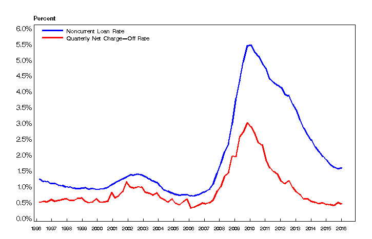
The historical US series illustrates this difference. It is not valid to infer a common denominator or annual horizon simply because both lines are percentages. The noncurrent series is a point-in-time stock ratio, whereas the displayed net-charge-off series is measured over a quarter using the source's convention. Timing and definitions must be checked before comparing their heights or using either as an estimate of prospective .
What historical lending-rate data show
The Swiss descriptive evidence below groups loans by size and product. The smallest displayed size class covers CHF 50,000–100,000 and the largest exceeds CHF 1 million; the intermediate classes are retained under their original labels because their precise cutoffs are not specified in this extract. Interest-rate columns are annual percentages. The observation count and share refer to the corresponding product's sample, not to the overall Swiss loan stock.
| Product | Size class | N | Sample share (%) | Mean (%) | Min (%) | 25th percentile (%) | Median (%) | 75th percentile (%) | Max (%) |
|---|---|---|---|---|---|---|---|---|---|
| Overdraft | 1 | 47,985 | 48.20 | 5.30 | 0.00 | 4.50 | 5.25 | 6.00 | 10.00 |
| Overdraft | 2 | 39,060 | 39.23 | 5.36 | 0.01 | 4.70 | 5.50 | 6.00 | 10.00 |
| Overdraft | 3 | 6,165 | 6.19 | 5.17 | 0.25 | 4.50 | 5.25 | 5.75 | 9.95 |
| Overdraft | 4 | 6,350 | 6.38 | 4.89 | 0.00 | 4.25 | 5.00 | 5.75 | 9.95 |
| Mortgage | 1 | 28,802 | 16.63 | 3.22 | 0.00 | 2.75 | 3.25 | 3.70 | 8.75 |
| Mortgage | 2 | 95,191 | 54.96 | 3.08 | 0.28 | 2.70 | 3.00 | 3.50 | 8.75 |
| Mortgage | 3 | 25,960 | 14.99 | 3.06 | 0.43 | 2.63 | 3.13 | 3.50 | 7.50 |
| Mortgage | 4 | 23,233 | 13.42 | 2.99 | 0.42 | 2.58 | 3.13 | 3.50 | 7.50 |
| Investment loan | 1 | 3,713 | 4.07 | 3.25 | 0.37 | 2.10 | 3.25 | 4.16 | 10.00 |
| Investment loan | 2 | 26,601 | 29.15 | 3.01 | 0.22 | 1.80 | 3.00 | 4.00 | 10.00 |
| Investment loan | 3 | 17,869 | 19.58 | 2.54 | 0.16 | 1.25 | 2.55 | 3.54 | 10.00 |
| Investment loan | 4 | 43,063 | 47.19 | 2.23 | 0.12 | 1.00 | 2.05 | 3.25 | 9.77 |
Mean investment-loan rates decline from 3.25% in class 1 to 2.23% in class 4, consistent with lower costs per franc for larger loans. The pattern is not strictly monotonic for every product, and it is not a controlled estimate of the causal effect of size. Borrower risk, collateral, maturity, bargaining and contract type also differ across groups. The minimum and maximum columns show that a class mean can conceal substantial dispersion.
| Product | Risk class | N | Sample share (%) | Mean (%) | Min (%) | 25th percentile (%) | Median (%) | 75th percentile (%) | Max (%) |
|---|---|---|---|---|---|---|---|---|---|
| Overdraft | 1 | 2,002 | 2.01 | 5.13 | 0.25 | 4.25 | 5.50 | 5.75 | 9.50 |
| Overdraft | 2 | 5,544 | 5.57 | 5.38 | 0.00 | 4.75 | 5.55 | 5.88 | 9.95 |
| Overdraft | 3 | 25,721 | 25.83 | 5.52 | 0.01 | 5.00 | 5.60 | 6.00 | 9.95 |
| Overdraft | 4 | 41,383 | 41.57 | 5.24 | 0.00 | 4.50 | 5.25 | 6.00 | 10.00 |
| Overdraft | 5 | 13,729 | 13.79 | 5.37 | 0.85 | 4.50 | 5.25 | 6.00 | 10.00 |
| Mortgage | 1 | 2,240 | 1.29 | 3.10 | 0.65 | 2.75 | 3.13 | 3.56 | 6.00 |
| Mortgage | 2 | 7,193 | 4.15 | 2.95 | 0.44 | 2.50 | 3.00 | 3.50 | 6.75 |
| Mortgage | 3 | 29,874 | 17.25 | 3.01 | 0.42 | 2.60 | 3.00 | 3.50 | 7.13 |
| Mortgage | 4 | 73,220 | 42.28 | 2.95 | 0.28 | 2.50 | 2.88 | 3.50 | 7.63 |
| Mortgage | 5 | 20,137 | 11.63 | 3.25 | 0.00 | 2.75 | 3.25 | 3.75 | 8.75 |
| Investment loan | 1 | 3,819 | 4.19 | 2.24 | 0.23 | 1.10 | 2.00 | 3.30 | 5.83 |
| Investment loan | 2 | 4,229 | 4.63 | 2.11 | 0.28 | 0.84 | 1.95 | 3.28 | 5.80 |
| Investment loan | 3 | 17,837 | 19.55 | 2.20 | 0.22 | 1.00 | 2.07 | 3.20 | 6.90 |
| Investment loan | 4 | 42,006 | 46.04 | 2.56 | 0.12 | 1.20 | 2.50 | 3.60 | 9.34 |
| Investment loan | 5 | 14,572 | 15.97 | 2.90 | 0.32 | 1.45 | 2.80 | 4.00 | 10.00 |
Class 1 denotes expected loss below 0.05% of exposure and class 5 expected loss above 2.6%; the intermediate class boundaries are not supplied here. Counts and percentages need not cover every observation in the size table, because an observation may lack a risk classification. In investment lending, the mean increases from 2.24% in class 1 to 2.90% in class 5, but the middle groups and the other products show why a raw average is not an exact pricing equation. Contract rates and expected losses can also be measured at different times.
Historical Swiss descriptive tables attributed to Cecchin (2011). Values are reproduced as historical observations, with the original class labels and the cutoffs actually provided; no unreported class boundaries or observation-level data have been inferred.
Debt funding, equity and a complete pricing calculation
Debt and equity supply funds in different ways. Depositors and other creditors have contractual claims; shareholders absorb residual losses and require compensation for that risk. A bank can allocate more equity capital to riskier exposures even though individual deposits and equity shares are not physically earmarked for particular loans. The allocation is a management representation of the loss-absorbing resources needed to support the asset, influenced by economic risk and regulatory constraints.
It is not valid to hold the required equity return fixed and conclude that reducing equity always creates a free saving. More leverage usually makes the remaining equity riskier, which can increase its required return. The cost of debt, distress costs, tax effects and constraints can also change. Similarly, expected loss should not be counted once as a loss allowance and again as an identical extra capital cost without explaining the convention.
Consider a EUR 1 million one-year loan with operating costs of EUR 5,000, and . The assigned funding is 90% deposits at 2% and 10% equity requiring 10%. Operating cost is 50 basis points, expected loss is 80 basis points and the weighted funding charge is . The additive required rate is therefore:
The corresponding annual revenue is EUR 41,000: EUR 5,000 for operations, EUR 8,000 for expected losses, EUR 18,000 for deposit interest and EUR 10,000 for the return on allocated equity. The last item is an economic required return, not an interest expense payable to shareholders in the profit-and-loss statement.
An exact cash-flow version illustrates why assumptions matter. Suppose the loan pays principal and its full coupon only if it survives to year-end, and a default instead returns at year-end with no coupon. Let and . Expected receipts must equal , giving:
Under these additional assumptions, the rate is , rather than 4.1%. The difference compensates for the coupon lost in default. Both calculations are understandable once their conventions are explicit; mixing the additive revenue convention with the terminal-default model silently produces an inconsistency.
Worked application: loan pricing and the bank's full income statement
Change the inputs to a EUR 1 million loan with EUR 5,000 operating cost, , , 90% deposit funding at 1% and 10% equity requiring 10%. Under the additive convention, the required rate is . Now suppose the bank starts the year with EUR 80 million of such loans and EUR 20 million of liquidity earning no interest. It is funded with EUR 90 million of deposits and EUR 10 million of equity, has no other revenue or costs and ignores taxes.
| Assets | Amount | Liabilities and equity | Amount |
|---|---|---|---|
| Liquidity | 20.00 | Deposits | 90.00 |
| Loans | 80.00 | Equity | 10.00 |
| Total assets | 100.00 | Total liabilities and equity | 100.00 |
| Item | Calculation | Amount |
|---|---|---|
| Interest income | 80 × 4.4% | 3.52 |
| Deposit interest expense | 90 × 1% | −0.90 |
| Net interest income | 3.52 − 0.90 | 2.62 |
| Loan-loss expense | 80 × 2% × 100% | −1.60 |
| Non-interest income | Assumed absent | 0.00 |
| Trading income | Assumed absent | 0.00 |
| Salary and administrative cost | 80 loans × EUR 5,000 | −0.40 |
| Profit before tax | 2.62 − 1.60 − 0.40 | 0.62 |
Profit of EUR 0.62 million on EUR 10 million of equity implies a pretax return of 6.2%, below the 10% required return. This is not a failure of arithmetic: the 4.4% rate was calibrated to the funding and equity allocated to the loan itself, while one-fifth of the bank's assets earns nothing. The loans support EUR 8 million of allocated equity and generate the corresponding EUR 0.8 million before the funding cost of the liquidity buffer. The buffer uses EUR 18 million of deposits costing EUR 0.18 million and EUR 2 million of equity, giving actual accounting profit of EUR 0.62 million and an economic shortfall of EUR 0.38 million relative to the whole bank's EUR 1 million target.
To achieve the whole-bank pretax target under the same additive assumptions, total loan revenue would have to cover million euros, requiring on the loans. Liquidity is useful despite its opportunity cost, so this result is a reason to price and allocate that cost explicitly, not to assume the bank should hold none. Under the alternative terminal-default convention, the original 4.4% quote would instead need to be for the isolated loan; its income statement would also need to use expected collected coupons consistently.
Borrower participation under limited liability
Now consider 2,000 applicants who each need an indivisible investment of 100 monetary units. Half are lower-risk borrowers with success probability and project proceeds on success. Half are higher-risk borrowers with and . Both receive zero on failure. Applicants know their types; the bank cannot distinguish them and cannot use a signal or collateral in this model. The bank has at most 100,000 units of funds, enough for 1,000 loans, and the risk-free funding rate is .
At the contractual lending rate , debt due is . A risk-neutral borrower of type receives the limited-liability payoff in the success state and zero otherwise. Expected private surplus is therefore:
The participation rule here requires strictly positive surplus. Lower-risk applicants borrow only for , while higher-risk applicants borrow for . At the threshold a borrower is indifferent and, by convention, does not apply. While both types participate, their expected surpluses are and . These linear expressions should not be extrapolated into negative private payoffs after limited liability binds; the borrower instead declines the loan.
The safer type has the higher expected project output, , compared with . Nevertheless, the riskier type is willing to accept a higher promised interest rate because its success-state upside is larger and repayment is required less often. A willingness to pay more is therefore not sufficient evidence that an applicant is a better credit risk.
Expected lender receipts and the correct supply intervals
Let denote the bank's expected gross repayment per loan of 100. When both groups apply, average success probability is . At 30% the safe borrowers leave, reducing this probability to 0.8. Consequently:
At rates of 35% or more there are no applicants under the strict-participation rule, so the bank makes no loans. Gross repayments are not profits: the bank must pay 105 per funded loan to cover principal and the 5% funding obligation. Expected net profit is . In particular, the break-even rate while both types apply is , not 23.52% exactly.
| Contract rate | Applicants | Mean success probability | Gross receipts | Profit after funding cost |
|---|---|---|---|---|
| 0% | 2000 | 0.85 | 85.0000 | -20.0000 |
| 5% | 2000 | 0.85 | 89.2500 | -15.7500 |
| 10% | 2000 | 0.85 | 93.5000 | -11.5000 |
| 15% | 2000 | 0.85 | 97.7500 | -7.2500 |
| 20% | 2000 | 0.85 | 102.0000 | -3.0000 |
| 23.5294…% | 2000 | 0.85 | 105.0000 | 0.0000 |
| 25% | 2000 | 0.85 | 106.2500 | 1.2500 |
| 29.99% | 2000 | 0.85 | 110.4915 | 5.4915 |
| 30% | 1000 | 0.80 | 104.0000 | -1.0000 |
| 31% | 1000 | 0.80 | 104.8000 | -0.2000 |
| 31.25% | 1000 | 0.80 | 105.0000 | 0.0000 |
| 34.99% | 1000 | 0.80 | 107.9920 | 2.9920 |
| 35% | 0 | No applicants | No loan | Not applicable |
| 40% | 0 | No applicants | No loan | Not applicable |
The first profitable interval is above approximately 23.5294% and below 30%. Immediately at 30%, gross receipts fall from nearly 110.5 to 104, so lending becomes unprofitable again. The high-risk-only pool breaks even at , and is profitable between 31.25% and 35%. At either break-even boundary the bank is indifferent; an explicit tie rule would determine how much it lends. A graph showing capacity of 1,000 loans at every rate above the first break-even threshold would therefore be incorrect.
Expected receipts rise toward 110.5 just below 30% and toward only 108 just below 35%. With a smallest rate increment of one basis point, the preferred offer is 29.99%, giving receipts of 110.4915 and profit of 5.4915 per loan. If rates were continuous and borrowers refused exactly at zero surplus, “just below 30%” would describe a supremum rather than an attained exact optimum. Stating the rate increment or participation convention removes this minor mathematical ambiguity.
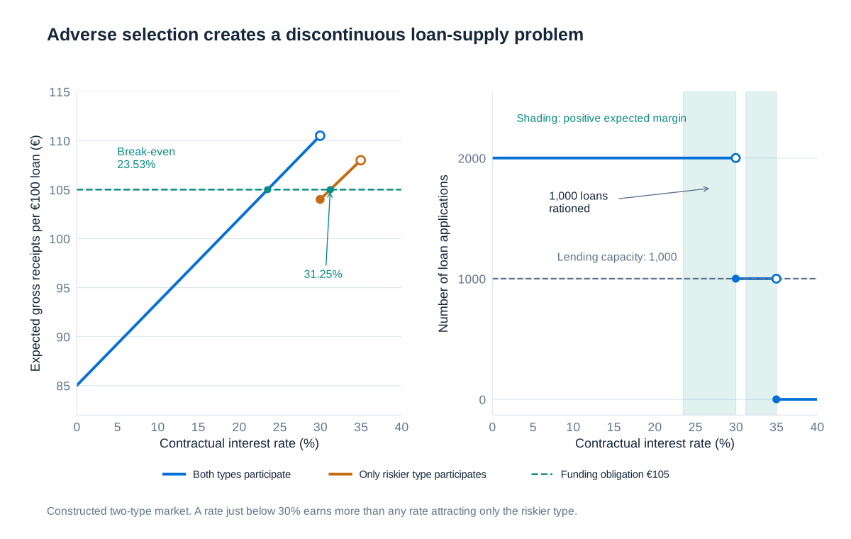
Why the bank rations credit instead of raising the rate
At 29.99%, all 2,000 applicants want loans, but the bank can finance only 1,000. With no additional way to distinguish applicants, it grants 1,000 loans and rejects 1,000 interested borrowers. Raising the rate to reduce demand changes the composition of applicants and lowers the bank's maximum expected receipts. Quantity rationing is therefore compatible with profit maximisation; the bank need not be subject to an externally imposed interest-rate ceiling.
An outright refusal to an applicant who accepts the offered terms is called type 1 rationing here. Granting less than the requested amount is type 2 rationing. If investment were perfectly divisible and payoffs scaled proportionally, the bank could distribute 50 units to each applicant rather than 100 to half of them. That alternative requires divisible productive opportunities; providing half the financing for an indivisible project may make the whole project impossible.
The finite funding capacity is part of this example. The wider Stiglitz–Weiss insight is that information and incentive effects can prevent the interest rate from clearing the credit market, even though some rejected applicants would accept the price. Rejection alone does not prove this mechanism: a borrower can also be denied because the project is unviable, legal conditions are unmet or the bank cannot assess repayment. Nor is every borrower who declines an expensive offer quantity-rationed. A precise analysis separates demand at the offered terms from the supply decision.
Alternatives include better screening, monitoring, collateral, guarantees, shorter maturities or relationships that reveal information. Each has costs and may change which customers can borrow. A collateral requirement can screen risk but exclude asset-poor applicants; more screening can improve decisions but be too costly for a small loan. The existence of a remedy in theory does not mean that credit rationing vanishes in practice.
Three worked variations on the rationing model
Keep 2,000 applicants, a loan size of 100, equal type shares and capacity for 1,000 loans, but set the funding rate to zero. In each variation, compare the bank's expected receipts near the participation cutoffs rather than assume that adverse selection always implies rationing. Rates written as a cutoff below mean the limit from below, or the closest feasible lower quote if the bank uses a discrete rate grid.
| Variation | Type I: success / failure proceeds and probability | Type II: success / failure proceeds and probability | Receipts with both types near the lower cutoff | Receipts with the remaining type near its cutoff | Preferred outcome |
|---|---|---|---|---|---|
| A | 130 / 0; p = 0.9 | 120 / 0; p = 0.8 | 0.85 × 120 = 102 near 20% | 0.9 × 130 = 117 near 30% | Only type I borrows; no quantity rationing |
| B | 130 / 80; p = 0.9 | 135 / 0; p = 0.8 | 0.5(0.9 × 130 + 0.1 × 80) + 0.5(0.8 × 130) = 114.5 near 30% | 0.8 × 135 = 108 near 35% | Both types apply; 1,000 applicants rejected |
| C | 130 / 0; p = 0.9 | 150 / 0; p = 0.8 | 0.85 × 130 = 110.5 near 30% | 0.8 × 150 = 120 near 50% | Only type II borrows; no quantity rationing |
In variation A, the safer borrower also has the higher success-state return. The riskier type exits around 20%, so an increase in the rate improves the applicant pool. Charging just below 30% attracts exactly the 1,000 safer applicants and produces receipts close to 117, more than the 102 available just below 20%. Every applicant willing to borrow at the selected rate receives a loan, even though the other type declines to apply. This is price selection rather than quantity rationing.
In variation B, the lower-risk project produces 80 even in its unsuccessful state. Near the 30% cutoff, the bank's expected receipt from this type is ; from the higher-risk type it is . Their average is 114.5. If the safe borrowers withdraw and the bank raises the rate toward 35%, receipts reach only 108. It prefers the lower rate and rationing. The 80-unit recovery must be included in bank receipts; it is not a payment retained by the borrower because the debt exceeds 80 in this region.
In variation C, adverse selection still occurs at 30%, but the riskier project's success-state proceeds are large enough to support a rate near 50%. Receipts of 120 exceed 110.5, so the bank chooses the high-risk-only pool and fills its 1,000-loan capacity without rejecting any willing applicant. Adverse selection is thus a mechanism that can cause rationing, not a sufficient condition for it. The lender must compare the entire expected-receipts schedule.
Empirical evidence on requested and granted credit
To study rationing, one needs to observe what borrowers requested as well as what banks granted. A database containing only completed loans cannot directly show whether a firm wanted more. Kirschenmann's study uses roughly 98,000 matched applications and contracts for micro and small businesses at a Bulgarian bank during 2003–2007. The firms had mean assets around EUR 35,000 and mean age around eight years; loans averaged approximately EUR 5,000 with maturity around 28 months. Firms appear in sequences of one to ten loans. Interest and collateral terms followed the bank's fixed contractual framework, which makes the approved amount an especially relevant adjustment margin.
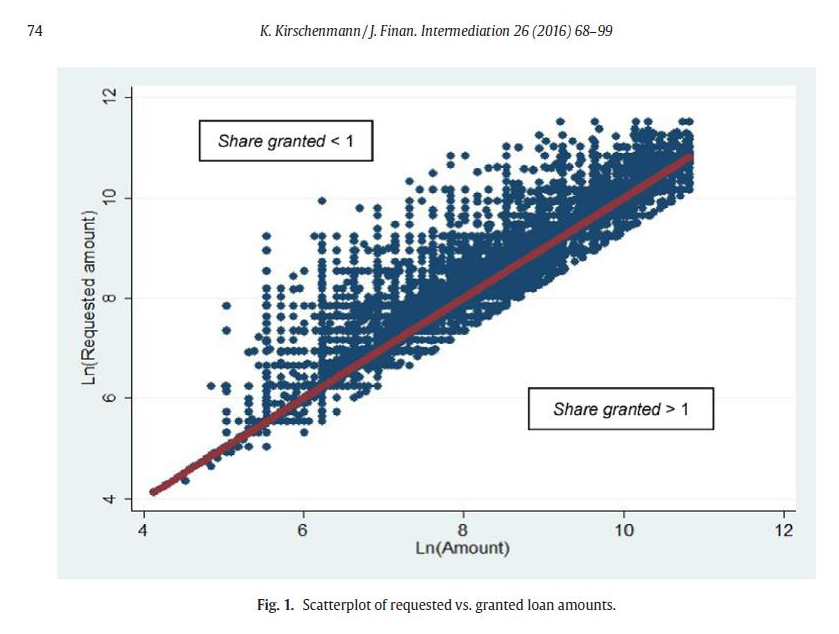
In the scatter, the horizontal axis is the logarithm of the granted amount and the vertical axis the logarithm of the requested amount. The 45-degree line means request equals grant. A point above it means the request exceeds the grant, so the granted share is below one. Logarithms show proportional differences; the vertical gap is the logarithm of the requested-to-granted ratio, not an amount in euros. Observations below the line have granted amounts exceeding the recorded request and should not be mistaken for rationing.
| Comparison | First loans: share granted | Later loans: share granted | Difference-in-differences |
|---|---|---|---|
| Initially young firms | 0.856***; SE 0.002; N = 11,428 | 0.938***; SE 0.003; N = 6,404 | Not separately reported |
| Initially old firms | 0.905***; SE 0.001; N = 41,933 | 0.954***; SE 0.001; N = 37,129 | Not separately reported |
| Young minus old | −0.050***; SE 0.002; N = 53,361 | −0.016***; SE 0.003; N = 43,533 | −0.033***; SE 0.004; N = 96,894 |
SE denotes standard error and N the number of observations. Three stars indicate significance at the 1% level in the reported table; the original convention also uses two stars for 5% and one for 10%. The first-loan gap means young firms receive about five percentage points less of their requested credit than old firms. The gap is narrower for later loans. The reported difference-in-differences uses the first-loan gap minus the later-loan gap, explaining its negative sign. Its value and the differences need not equal subtraction of the rounded displayed means exactly.
The wider evidence finds more rationing for young, small and previously unbanked firms and a reduction over repeated borrowing. This is consistent with information accumulation, but descriptive associations do not by themselves identify a single causal explanation. Continuing borrowers are a selected group; collateral, risk, profitability and requested amounts may change with experience. The result supports the importance of opacity and relationship history without proving that every reduction in rationing is caused by private information alone.
Karolin Kirschenmann (2016), Credit rationing in small firm-bank relationships, Journal of Financial Intermediation 26, 68–99. Table values and the scatter refer to this historical sample, not to all firms or present-day Bulgarian lending.
Two banks and the winner's curse of uninformed lending
Suppose half the applicants always repay and half never repay. Bank 1 has perfect screening and can distinguish the types; Bank 2 cannot. Each bank simultaneously chooses whether to offer a loan and its rate, capped at 200%, and a repayable borrower prefers a lower rate. For the following calculation, normalise principal to one and set the funding cost to zero. Screening costs, capacity constraints and borrower surplus limits are ignored. Tie-breaking and how non-repaying applicants choose between offers matter for a full game-theoretic solution.
Without a competitor, the uninformed bank would break even at 100% interest because . It might therefore believe that offering 100% to everyone is safe. But the relevant repayment probability is conditional on winning the customer. Bank 1 can offer 99% only to good borrowers and decline bad borrowers. Good customers choose Bank 1; Bank 2 is left with the non-repaying group and receives zero. The applicant pool before competition is not the pool that accepts the uninformed bank's offer afterward.
The offer “Bank 1 lends to good applicants at 99%; Bank 2 stays out” is useful for understanding entry deterrence. To win good customers by undercutting 99%, Bank 2 must quote a rate at which even the original half-good pool is loss-making. A higher offer loses the good borrowers to the informed bank. Bank 1 can earn an information rent even though Bank 2 is potentially available as a competitor.
However, that offer pair is not a Nash equilibrium of the simultaneous game as stated. If Bank 2 has already chosen no offer and that strategy is held fixed, Bank 1 can profitably raise its rate to the permitted cap for the good borrowers. Conversely, sufficiently high pricing by Bank 1 would invite a profitable undercutting offer from Bank 2 when the original pool includes enough good customers. A complete equilibrium analysis needs explicit borrower payoffs and tie rules and may require mixed strategies. The 99% example is an explanation of the information problem, not a solved equilibrium that should be presented as one.
The economically durable conclusions are that information has value, that avoiding a market can be rational for a poorly informed lender, and that a bank's profit depends on its information advantage relative to competitors. Knowing what other lenders know can be as important as knowing the unconditional average default rate. This is the credit-market version of a winner's curse: winning business can itself be bad news when a better-informed competitor declined it.
How relationship banking changes information and incentives
Relationship banking develops when repeated interactions provide the lender with private information about a borrower. Repeated loans reveal repayment behaviour and the reliability of earlier forecasts. Cross-selling, such as providing the operating account as well as a loan, reveals incoming receipts, payment obligations and changes in liquidity. Such information can be “soft”: knowledge of management competence or customer stability may be valuable even when it cannot be reduced to a public, verifiable score.
Information accumulation can reduce adverse selection, while the prospect of future access to credit can reduce moral hazard. An entrepreneur may work harder and avoid excessive risk when poor behaviour threatens a continuing valuable relationship. The bank may also distinguish a temporary cash-flow shock from a deteriorating business more effectively than a new outside lender. These benefits are strongest when monitoring is credible and continuation depends on repayment and performance rather than unconditional support.
| Country | Firms (N) | Mean relationships | Median | Maximum | One bank (%) | Two banks (%) | Three to seven (%) | More than seven (%) |
|---|---|---|---|---|---|---|---|---|
| Italy | 64 | 15.2 | 12 | 70 | 3.1 | 3.1 | 23.4 | 70.3 |
| Portugal | 39 | 11.5 | 10 | 40 | 5.1 | 2.6 | 30.8 | 61.5 |
| France | 24 | 11.3 | 9 | 50 | 4.2 | 4.2 | 33.3 | 58.3 |
| Belgium | 8 | 11.1 | 7 | 30 | 0.0 | 25.0 | 25.0 | 50.0 |
| Spain | 68 | 9.7 | 7 | 60 | 1.5 | 7.4 | 44.1 | 47.1 |
| Germany | 63 | 8.1 | 5 | 29 | 15.9 | 7.9 | 39.7 | 36.5 |
| Greece | 37 | 7.4 | 6 | 19 | 0.0 | 8.1 | 51.4 | 40.5 |
| Austria | 36 | 5.2 | 3 | 22 | 19.4 | 13.9 | 44.4 | 22.2 |
| Luxembourg | 7 | 5.0 | 4 | 18 | 28.6 | 0.0 | 57.1 | 14.3 |
| Czech Republic | 58 | 4.7 | 4 | 14 | 3.4 | 10.3 | 70.7 | 15.5 |
| Switzerland | 36 | 3.6 | 2 | 40 | 41.7 | 19.4 | 30.6 | 8.3 |
The historical corporate comparison shows that relationship lending need not mean having only one bank. In the displayed Italian sample, the median firm had 12 relationships; in the Swiss sample it had two. The distinction between a mean and a median matters because a few firms with many banks can raise the mean substantially. The small country samples and historical setting limit generalisation, and the percentages can differ slightly from 100 because of rounding. Maintaining several banks can diversify funding risk and bargaining options, while still allowing one bank to be the principal relationship lender.
Corporate relationship data: Ongena and Smith (2000), historical cross-country sample. The table reproduces the countries and variables available in the supplied excerpt; it is not a current census of European firms.
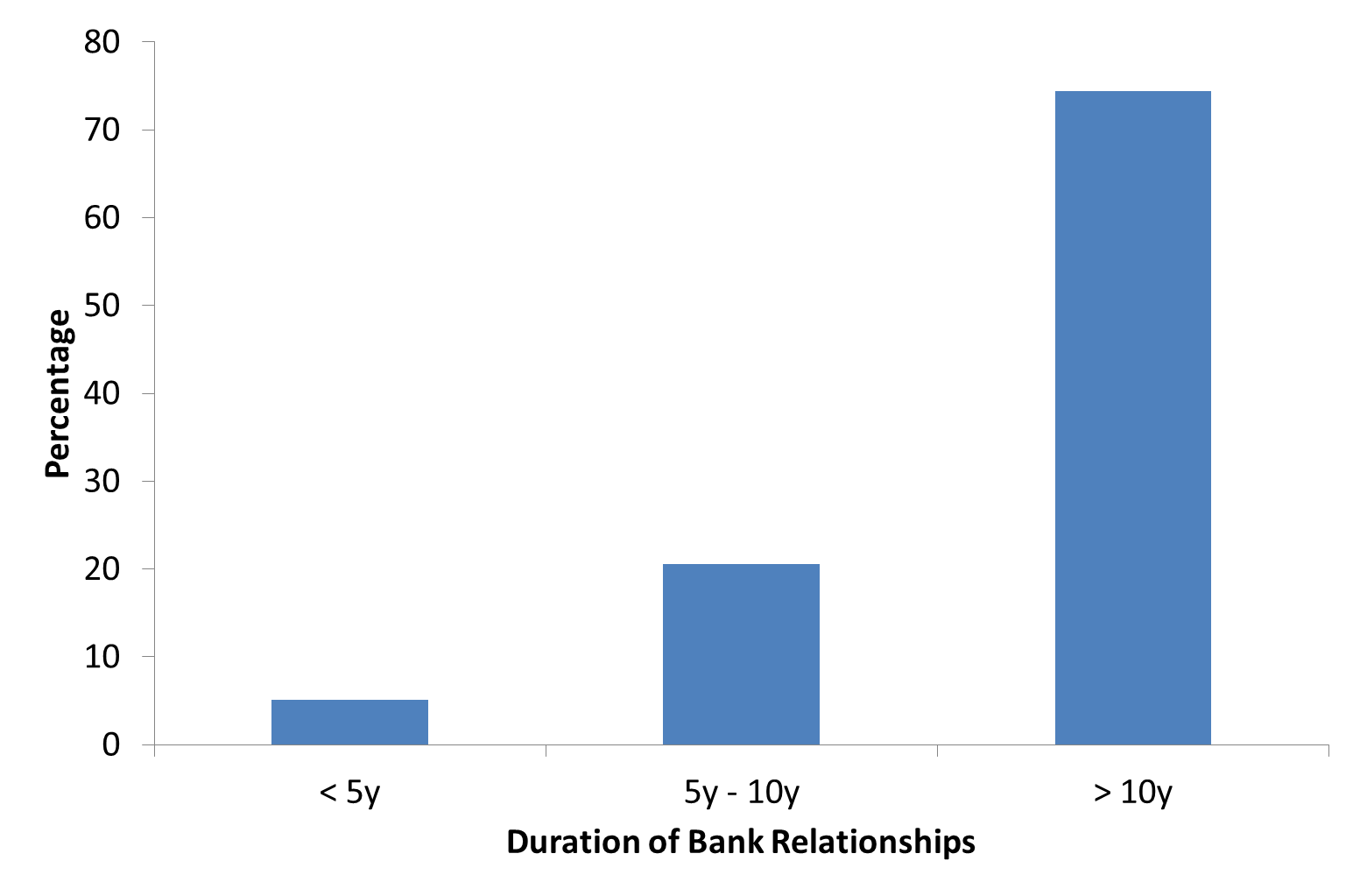
Household relationships can also persist for many years. The historical sample in the duration chart contains 2,644 bank relationships belonging to 1,456 households, so the observational unit is a relationship rather than a unique person. Most relationships in the chart lasted more than ten years. The difference between the number of households and relationships also shows that households can use several banks at once.
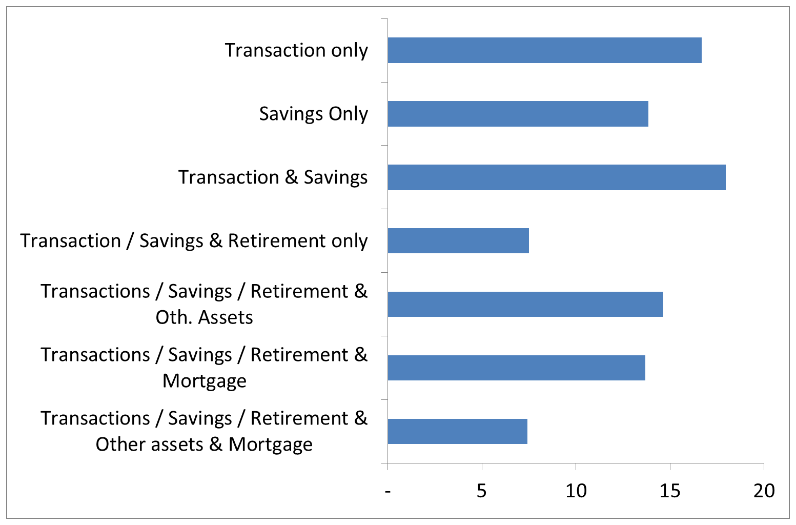
The product-scope chart describes combinations of transactions, savings, retirement products, other assets and mortgages. A broad relationship can supply the bank with information across several financial activities, while also increasing the customer's switching effort. The categories describe product bundles, not an ordering from “good” to “bad” customers. Their historical proportions must not be treated as individual borrowers' credit scores or evidence that cross-selling automatically improves welfare.
Historical household relationship charts attributed to Brown and Hoffmann (2016 for duration; 2013 for product scope), using 2,644 relationships of 1,456 households. Approximate visual heights are not converted into invented exact observations.
The benefits and costs of an informed incumbent
A relationship can improve access to credit, reduce repeated screening costs and allow useful flexibility during temporary difficulty. But private information also creates a potential hold-up problem: outside banks may fear that a borrower seeking to switch is one the incumbent knows to be weak. The incumbent can then gain pricing power because competitors cannot reproduce its information cheaply. The two-bank example explains why more nominal competitors do not guarantee equal information or aggressive price competition for every customer.
Other risks include dependence on one bank's funding health, conflicts across the bank's advisory and lending roles, and excessive forbearance when a lender protects an existing exposure by advancing more funds to a weak borrower. Multiple relationships, transferable information, credit registries and transparent financial reporting can limit these costs, but they can also reduce each bank's incentive to invest in proprietary monitoring. The appropriate structure balances information production, competition and continuity rather than treating either transactional lending or relationship banking as universally superior.
The main connection is that pricing, quantities and information are jointly determined. A higher coupon may compensate for a given risk, yet also change that risk through selection and incentives. A longer relationship may improve screening, yet create market power. Sound lending therefore assesses the entire contract and customer relationship: expected cash flows, operating and funding costs, capital, collateral, information and the consequences of competing offers.
5. Investment Banking, Syndication and Securitisation
Investment banking connects companies that need capital with investors willing to supply it. The intermediary may advise on an acquisition, arrange a syndicated loan, underwrite a bond or share issue, distribute securities, or structure claims against a portfolio of loans. These activities complement commercial banking: the same banking group may hold a corporate loan, organise its distribution and later advise the borrower on refinancing. Understanding the economic function therefore requires following the cash flows, information and contractual obligations, rather than relying on the institution’s name.
Three arrangements illustrate these connections. Syndication spreads one borrower’s financing among several lenders. Securitisation pools assets and reallocates their cash flows among investors with different priorities. Acquisition finance coordinates commitments and permanent funding across the uncertain interval between agreeing a transaction and completing it. Each can improve access to finance, but each also creates an agency problem: the intermediary arranging a transaction may know more than the investors who ultimately bear its risk.
Investment-banking services and what league tables measure
Corporate-finance services cover mergers and acquisitions, equity and debt issuance, and syndicated lending. Research helps clients interpret companies, securities and markets; securities and derivatives trading provides execution, market making and risk transfer. Investment management serves private wealth and institutional portfolios. These functions bring issuers and investors together but need not all be undertaken by the same legal entity. An underwriter committing to buy an issue bears a different risk from an adviser paid for advice or a distributor operating on a best-efforts basis. Revenue from fees also differs from the profits and losses generated by holding trading inventory or loans.
Combining services can create conflicts of interest. An intermediary may advise an issuer while selling securities to investors, financing a bidder or trading related instruments. Confidential information, research independence, disclosure and clear allocation of responsibilities matter because the clients do not necessarily share the same objectives. A successful distribution is not by itself evidence that the product suits every buyer.
League tables rank activity under a defined methodology. The historical table below records investment-banking fee estimates for calendar 2024, in a snapshot dated 10 July 2025. It illustrates differences in business mix: some institutions earned a larger proportion from merger advice, others from bonds or loans. The “market total” is the total reported market, not the sum of the ten institutions. Rounded product percentages need not sum exactly to 100. Neither gross fees nor a high rank demonstrates superior profitability, capital efficiency or advice quality.
| Institution | Fees, USD m | Change | M&A share | Equity share | Bonds share | Loans share |
|---|---|---|---|---|---|---|
| JPMorgan | 9,373.98 | +27% | 32% | 17% | 24% | 27% |
| Goldman Sachs | 7,261.67 | +23% | 47% | 17% | 19% | 16% |
| BofA Securities | 6,624.60 | +27% | 22% | 14% | 29% | 35% |
| Morgan Stanley | 5,903.70 | +33% | 38% | 24% | 23% | 15% |
| Citi | 4,740.90 | +30% | 26% | 17% | 34% | 24% |
| Barclays | 3,538.96 | +18% | 23% | 14% | 36% | 26% |
| Wells Fargo | 2,781.51 | +30% | 12% | 8% | 39% | 40% |
| BNP Paribas | 2,498.77 | +25% | 14% | 6% | 49% | 32% |
| RBC Capital Markets | 2,428.66 | +22% | 23% | 8% | 35% | 34% |
| Jefferies | 2,421.11 | +49% | 46% | 22% | 10% | 22% |
| Reported market total | 120,764.79 | +17% | 29% | 13% | 33% | 25% |
Historical data: Financial Times investment-banking league-table snapshot, 10 July 2025, covering 1 January–31 December 2024. This dated illustration is not a current ranking.
A syndicated loan as a coordinated lending contract
A syndicated loan is credit granted by a group of lenders to one borrower under a common agreement. A mandated lead arranger negotiates the principal terms and coordinates the transaction. The bookrunner seeks commitments and allocates amounts among participants; an administrative agent handles notices, payments and contractual administration. Participating lenders provide agreed shares of the funding and normally have separate claims against the borrower. Lenders within the same tranche generally rank equally, but a facility can contain tranches with different currencies, maturities, security or priorities. “One agreement” does not mean that every lender jointly guarantees every other lender’s obligations.
Syndicated lending lies between bilateral relationship lending and bond finance. A bilateral loan is negotiated with one lender and is often comparatively easy to amend; it can nevertheless be transferable subject to consent and other restrictions. Syndicated loan interests often trade in a secondary market, though transfer restrictions and settlement frictions matter. Bonds normally offer greater standardisation and potentially wider distribution, while renegotiation may be harder when ownership is dispersed. Liquidity is a matter of degree: neither a bond listing nor a loan’s legal transferability guarantees an active market.
| Feature | Bilateral loan | Syndicated loan | Bond |
|---|---|---|---|
| Initial financing relationship | Borrower and one lender | Borrower and coordinated lender group | Issuer and securities investors |
| Typical information channel | Private lender information | Shared contractual reporting to lenders | Offering and continuing disclosures |
| Amendments | Direct negotiation | Contractual voting and consent thresholds | Security terms and bondholder consent rules |
| Transfer | May be restricted | Often permitted subject to agreement | Generally transferable, with market liquidity varying |
The historical Starwood Hotels & Resorts Worldwide facility shows how titles correspond to functions. A USD 250 million, two-year term loan signed on 30 May 2001 was arranged for general corporate purposes. Its quoted margin was LIBOR plus 125 basis points, with a 17.5-basis-point commitment fee. Deutsche Bank acted as mandated arranger, bookrunner and administrative agent; the participant group included Deutsche Bank, Bank One, Citibank, Crédit Lyonnais and UBS. The arranger designed and syndicated the transaction, whereas participants supplied funds. A commitment fee compensates for making capacity available under the specified contract; it should not automatically be applied to the same base as interest on outstanding principal.
Why borrowers, arrangers and participants choose syndication
For a borrower, syndication can replace numerous separate negotiations with a coordinated facility, increase the amount available and improve the combination of price and non-price terms. Private reporting to lenders can also preserve commercial confidentiality compared with a public securities offering. This is relative confidentiality, not freedom from all disclosure: listed issuers may still have legal reporting duties, and lenders require substantial information. A common agreement makes amendment possible without negotiating entirely separate contracts, although voting thresholds and conflicting lender interests can still obstruct restructuring.
For the arranger, a large loan may exceed an economic concentration limit or an applicable regulatory exposure limit if retained in full. Distribution reduces the retained exposure, earns arrangement and underwriting fees, and can support a wider client relationship. For participants, the deal offers diversification across borrowers, sectors or countries and uses lending capacity that their own origination network may not fill. It can also establish new client relationships. These benefits are conditional: buying another loan in an already crowded sector does not diversify that bank merely because the loan is syndicated.
The arranger’s information advantage creates a delegated-screening problem. Participants may rely excessively on the arranger, while an arranger planning to distribute most of the exposure may have weaker incentives to investigate. Retained exposure, reputation, contractual information duties and the participants’ own diligence help align incentives. Non-bank lenders, including collateralised loan obligations and investment funds, are particularly important in lower-rated term loans. Their participation redistributes credit risk away from deposit-funded banks, but banks may remain exposed through retained loans, underwriting commitments, credit lines and relationships with the new holders.
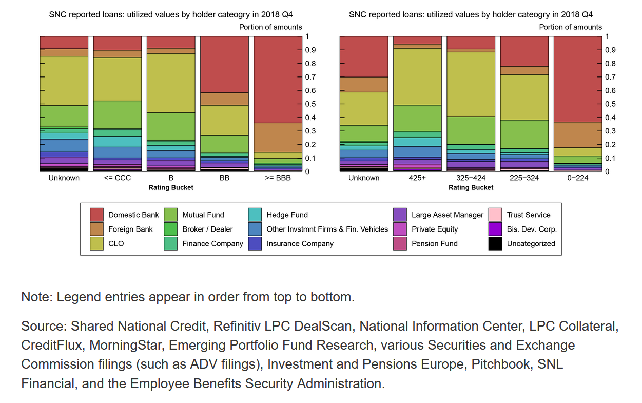
A historical 2024 market estimate placed global syndicated lending near USD 5.9 trillion, including approximately USD 3.9 trillion in the Americas, USD 1.0 trillion in Europe and USD 0.6 trillion in Asia-Pacific excluding Japan; the selected regional categories are not an exhaustive decomposition. Large reported transactions in 2024–25 included ByteDance’s USD 10.8 billion refinancing and Nippon Steel’s acquisition financing, with a JPY 2 trillion bridge and subsequent JPY 800 billion subordinated funding. PIF’s USD 15 billion revolving facility, announced in August 2024, involved 23 international institutions and replaced its 2021 facility. These examples distinguish refinancing existing debt, funding an acquisition and maintaining general liquidity: the same broad contractual form can serve different purposes.
The holdings figure is a historical Federal Reserve analysis of 2018 Q4: The U.S. Syndicated Term Loan Market: Who holds what and when? The market-volume and ByteDance/Nippon examples are dated LSEG/Reuters estimates; PIF confirms its facility in its August 2024 announcement.
Reading performance pricing: the eBay facility
A revolving credit facility promises access to borrowing up to an agreed limit, with drawings and repayments governed by the agreement. Commitment and utilisation are therefore different quantities. eBay’s agreement dated 22 November 2011 provided a USD 3 billion revolver, with JPMorgan as administrative agent and several arranging and agency banks. Its pricing grid linked the interest margin and commitment fee to the borrower’s debt ratings. A basis point is 0.01 percentage points: a margin of 0.625% is 62.5 basis points, added to the relevant benchmark rather than substituted for it.
| Level and rating category | Eurocurrency margin | Alternative base-rate margin | Commitment fee |
|---|---|---|---|
| I: at least AA− / Aa3 | 0.625% | 0.000% | 0.050% |
| II: A+ / A1, below I | 0.750% | 0.000% | 0.060% |
| III: A / A2, below I–II | 0.875% | 0.000% | 0.080% |
| IV: A− / A3, below I–III | 1.000% | 0.000% | 0.100% |
| V: below IV | 1.125% | 0.125% | 0.150% |
The rating labels summarise the S&P/Fitch and Moody’s categories shown in the historical agreement; the contract’s rules resolve split ratings. The agreement also required consolidated interest coverage of at least 3.00 times at each fiscal-quarter end. Interpreting that requirement needs the agreement’s definitions of earnings, interest expense and the consolidation perimeter. A ratio with the same name in a financial database may use a different numerator or denominator.
Benchmark continuity is another contractual issue. If the published reference rate disappears, the parties need a fallback, replacement mechanism or amendment; a quoted spread alone cannot determine interest. LIBOR in these historical examples is not a current available benchmark: the final synthetic settings ceased after 30 September 2024. Modern agreements commonly specify alternative benchmarks, associated conventions and adjustment mechanisms. The economic lesson is to read the benchmark clause, day-count convention, margin, fees, floor and fallback together.
Historical contract: eBay credit agreement dated 22 November 2011. For benchmark cessation, see the FCA’s confirmation of the end of LIBOR.
Why pricing grids and covenants are complements
Performance pricing changes the cost of debt as measured credit quality changes. It rewards stronger finances with a lower spread and increases compensation when leverage rises, earnings weaken or ratings fall. It can also screen applicants: a borrower privately expecting deterioration has less reason to accept a sharply increasing future spread. Managerial optimism can influence the perceived attractiveness of such a contract, but it is not valid to assume that every manager is overoptimistic. The mechanism works only to the extent that the chosen metric is informative and sufficiently resistant to manipulation.
| Level | Spread over LIBOR | Debt-rating category | Interest-coverage range |
|---|---|---|---|
| 1 | 0.30% | A2 / A or higher | At least 6.25 times |
| 2 | 0.35% | A3 / A− | At least 5.75, below 6.25 |
| 3 | 0.40% | Baa1 / BBB+ | At least 5.00, below 5.75 |
| 4 | 0.55% | Baa2 / BBB | At least 4.50, below 5.00 |
| 5 | 0.65% | Baa3 / BBB− | At least 3.75, below 4.50 |
| 6 | 0.80% | Below Baa3 / BBB− | Below 3.75 |
The same historical agreement imposed a maximum contract-defined leverage ratio of 0.62 and minimum interest coverage of 3.25 times. The grid’s lowest coverage band starts below 3.75, while the covenant is breached below 3.25; these thresholds are related but not identical. Pricing handles a range of deterioration while the covenant provides a separate intervention point. A breach can trigger consent requirements, renegotiation, restrictions or contractual remedies; it does not automatically mean immediate liquidation.
Why not simply keep increasing interest rates? Higher interest expense can further reduce coverage and creditworthiness, prompting another rate increase. At sufficiently severe distress, this feedback can damage repayment capacity rather than protect lenders. Covenants let the parties address behaviour and control rights instead of relying only on price. Short maturities are an imperfect substitute: refinancing frequently allows repricing and reassessment, but exposes the borrower to the possibility that funding disappears entirely. This rollover risk is different from paying a pre-agreed higher spread. Short-term lending is particularly relevant where detailed performance metrics or enforceable covenants are difficult to apply.
From loan origination to asset-backed securities
Securitisation converts cash flows from an asset pool into securities. In a typical cash transaction, an originator sells receivables to a special-purpose vehicle, which finances the purchase by issuing notes. Borrowers continue to make principal and interest payments; the servicer collects these and administers defaults, while a trustee or paying agent distributes amounts according to the contract. An underwriter helps design and place the securities. Credit enhancement may come from subordination, excess collateral, reserves or a third-party guarantee, for which a fee may be charged. Fees reduce the resources ultimately available to investors and must be included in valuation.
The vehicle and the underwriter are distinct roles, even when related companies perform several functions. Asset isolation depends on legal structure, enforceability and insolvency treatment, not merely on calling an entity “special purpose”. Accounting derecognition and regulatory capital relief also require their own conditions. Synthetic securitisations transfer specified credit risk without necessarily selling the underlying loans. In either form, risk transfer should be assessed economically: retained junior tranches, liquidity commitments or implicit support can leave the originator exposed.
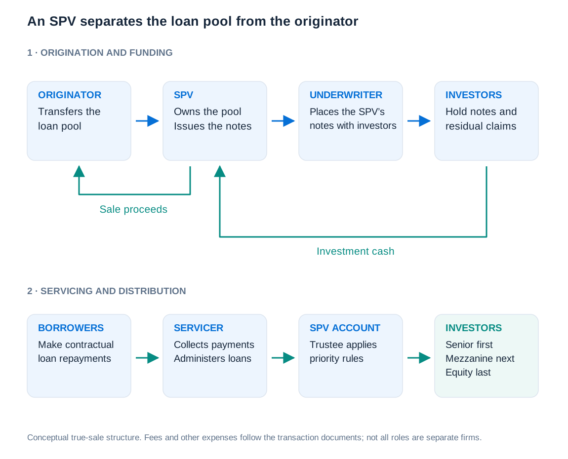
| Category | Typical underlying claims | Interpretive distinction |
|---|---|---|
| RMBS | Residential mortgages | Residential mortgage-backed securities |
| CMBS | Commercial property mortgages | Cash flows depend on commercial borrowers and property income |
| CLO | Corporate loans | A collateralised loan obligation is commonly treated as a form of CDO |
| CBO / broader CDO | Bonds or other debt claims | Collateralised bond/debt obligations describe the collateral mix |
| ABS in the narrower sense | Auto and consumer loans, credit cards, equipment leases, student loans and trade receivables | Excludes categories separately reported as MBS or CDO/CLO |
| Specialised receivables | Dealer floorplans, insurance premiums, aircraft leases, film or health-care receivables, music royalties and lottery payments | Requires pool-specific legal and cash-flow analysis |
“ABS” can therefore be an umbrella term for asset-backed securities generally or a narrow statistical category. Life-insurance-related claims and externally guaranteed, or “wrapped”, securities add other risks, including insurance-event assumptions and guarantor creditworthiness. The label alone does not establish the quality, maturity or liquidity of the investment.
Reading securitisation market statistics without mixing stocks and flows
Issuance measures securities created during a period; outstanding volume measures securities still in existence on a date. A stock accumulates past issuance net of repayments and other changes. Currency, geographic coverage and classification must match before comparing totals. Agency mortgage securities are especially important in the United States, reflecting the role of agency/GSE-related mortgage finance, whereas European classifications separately identify substantial SME and other collateral pools.
| Collateral category | Issuance |
|---|---|
| ABS | 62.7 |
| CDO/CLO | 49.2 |
| CMBS | 2.8 |
| RMBS | 120.4 |
| SME | 9.8 |
| Corporate | 0.0 |
| Total | 244.9 |
| Collateral category | Issuance |
|---|---|
| ABS | 280.1 |
| CDO | 78.2 |
| Agency MBS | 1,122.4 |
| Non-agency CMBS | 46.3 |
| Non-agency RMBS | 21.3 |
| Total reported | 1,548.4 |
The regional classifications differ, so categories with similar names should be checked before comparison. The published US total differs by 0.1 from the sum of rounded components. For outstanding securities, the retained historical snapshots are deliberately dated separately below. They cannot be interpreted as a same-date comparison or as growth from one region to the other.
| Collateral | Outstanding |
|---|---|
| Auto | 71.9 |
| Cards | 26.0 |
| SME ABS | 114.4 |
| CMBS | 29.8 |
| Consumer | 88.1 |
| Leases | 10.6 |
| RMBS | 539.0 |
| Other | 47.1 |
| Total excluding CLO/CDO, reported | 926.8 |
| CLO/CDO | 235.6 |
| Total including CLO/CDO | 1,162.4 |
| Collateral | Outstanding |
|---|---|
| ABS | 1,386.5 |
| Agency MBS | 8,134.8 |
| Non-agency RMBS | 734.4 |
| Non-agency CMBS | 588.4 |
| Total | 10,844.1 |
Historical AFME/SIFMA data; European component totals may differ by 0.1 due to rounding. The AFME Q1 2025 historical data snapshot confirms calendar-2024 issuance totals of EUR 244.9 billion for Europe and EUR 1,548.4 billion for the United States. The older US stock appears in AFME’s historical outstanding-volume tables, denominated in EUR billion.
Tranche priorities, attachment points and the loss waterfall
Tranching creates different claims against the same pool. Senior investors receive priority; mezzanine investors absorb losses after the first-loss position is exhausted; the equity tranche receives the residual. Seniority can support a high credit rating but does not automatically imply AAA or eliminate risk. The equity tranche may have a high expected return, yet it is a residual claim, not necessarily debt paying a guaranteed high coupon. Actual waterfalls also allocate fees, interest and principal separately, and performance triggers can redirect cash away from junior investors before final principal losses occur.
Before the global financial crisis, one attraction of tranching was the ability to create a large highly rated senior layer from assets of more moderate individual credit quality, alongside small riskier layers. Demand from institutions seeking highly rated securities helped support this market. The rating depended on subordination and model assumptions about the pool; it did not turn the underlying borrowers into safer borrowers. Errors about common shocks or recoveries could therefore undermine even a thick senior tranche.
Let be the initial pool principal, cumulative losses as a fraction of that principal, and and the tranche’s attachment and detachment points. The tranche has principal . Its loss amount and loss fraction are:
Attachment is the loss buffer beneath the tranche; detachment is the loss level exhausting it. All three percentages must use the same pool denominator. In a pool of 100 with equity of 3, mezzanine of 7 and senior claims of 90, the attachment/detachment pairs are 0%/3%, 3%/10% and 10%/100%. If loans of 10 default with loss given default of 40%, the pool loses 4, not 10. Equity loses its entire 3; mezzanine loses 1, or ; senior loses nothing. The pool’s surviving principal is 96 and the surviving tranche principals sum to the same 96.
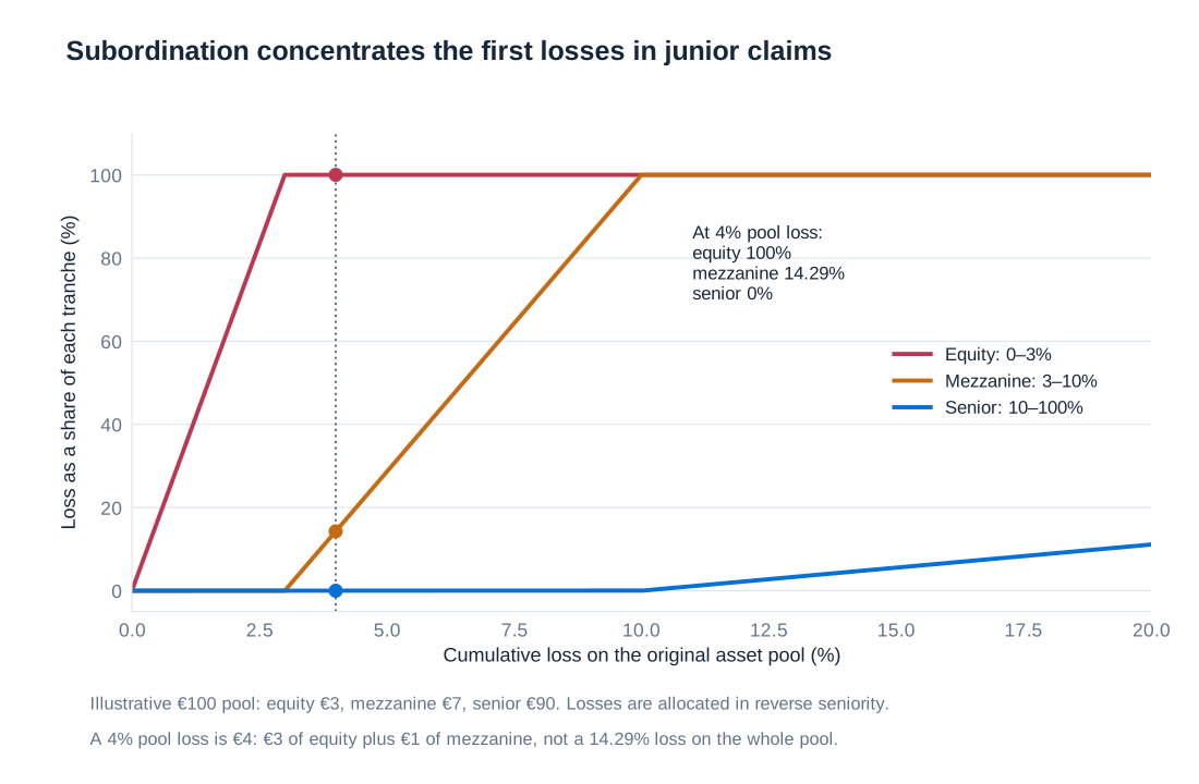
A second worked example uses a EUR 100 million pool with a 0–5% equity tranche, a 5–15% mezzanine tranche and an 85% senior tranche. With a 9% pool loss, mezzanine loses 4% of pool principal, which is 40% of its own principal. With EUR 12 million of losses, equity absorbs 5 and mezzanine 7; the mezzanine loss rate is 70%. With EUR 18 million of losses, both junior layers are exhausted and senior loses EUR 3 million, or . These calculations use different tranche boundaries from the preceding example and must not be mixed.
| Pool loss | Equity loss | Mezzanine loss | Senior loss | Mezzanine principal lost |
|---|---|---|---|---|
| 3 | 3 | 0 | 0 | 0% |
| 9 | 5 | 4 | 0 | 40% |
| 12 | 5 | 7 | 0 | 70% |
| 15 | 5 | 10 | 0 | 100% |
| 18 | 5 | 10 | 3 | 100% |
| 20 | 5 | 10 | 5 | 100% |
A complete two-loan securitisation calculation
Consider two one-year loans of EUR 100 each, both with zero contractual interest. Loan 1 has default probability 5%, loan 2 has default probability 10%, and recovery in default is 50% for each. Defaults are independent. Consequently, each loan pays either EUR 100 or EUR 50, and the pool pays EUR 200, EUR 150 or EUR 100. The probabilities multiply because independence is an explicit assumption; mere similarity of borrowers would not justify it.
| Outcome | Probability calculation | Probability | Pool payoff | Senior payoff | Equity payoff |
|---|---|---|---|---|---|
| Neither defaults | 85.5% | EUR 200 | EUR 130 | EUR 70 | |
| Only loan 1 defaults | 4.5% | EUR 150 | EUR 130 | EUR 20 | |
| Only loan 2 defaults | 9.5% | EUR 150 | EUR 130 | EUR 20 | |
| Both default | 0.5% | EUR 100 | EUR 100 | EUR 0 |
The senior claim fails to receive its full EUR 130 only when both loans default, so its default probability is 0.5%. Under the deliberately simplified rating mapping below it is classified Baa. The mapping is an illustrative exercise convention, not an agency’s general rating methodology: actual ratings also depend on horizon, instrument structure and other criteria. The quoted rounded intervals leave small gaps; these do not affect a probability of exactly 0.5% and should not be treated as a complete classification algorithm.
| Rating label | Quoted one-year default-probability range |
|---|---|
| Aaa | At most 0.02% |
| Aa | 0.03%–0.10% |
| A | 0.11%–0.24% |
| Baa | 0.25%–0.58% |
| Ba | Above 0.58% |
The pool’s expected loss is euros. Senior expected loss is euros, leaving EUR 7.35 expected loss for equity. Expected payoffs are therefore EUR 129.85 and EUR 62.65, which sum to EUR 192.50. A low probability of senior default should not be confused with no loss severity: conditional on default in this example, senior loses of principal.
Correlation and why expected pool loss is insufficient
Pool valuation depends on tranche boundaries, interest earned on assets, expected losses and the joint distribution of losses. With many independent risks, diversification makes realised average losses concentrate around their expectation. Common exposure to a region, industry or macroeconomic shock can instead produce many simultaneous defaults. The analogy is averaging independent dice rolls versus making every die show the same result: identical individual distributions need not produce the same distribution of the average.
The two-loan example makes this precise. Keep each loan’s default probability and recovery fixed, and write for the probability that both default. The four probabilities become , , and , with . Independence gives ; positive dependence raises it. Expected pool payoff remains EUR 192.50, but senior expected payoff is , and equity expected payoff is . A larger probability of joint default therefore transfers expected payoff from senior to equity in this structure. Equity benefits from more probability of the no-loss outcome while its downside is capped at zero.
This comparison holds marginal default risks fixed. It is not a claim that an economic crisis helps every equity-tranche investor: a crisis may raise default probabilities, lower recoveries, impair liquidity and change discount rates simultaneously. Nor does the direction for mezzanine tranches have to be monotonic. Tranche prices require the full distribution and pricing assumptions; an expected-loss calculation alone is not a market valuation.
Risk transfer, incentives and financial stability
For an originator, securitisation can release funding, diversify credit exposure and allow greater specialisation in origination, credit assessment and servicing. It may reduce interest-rate or liquidity mismatches when long-lived assets are funded by appropriately matched securities. It can also reduce regulatory capital requirements when the applicable risk-transfer conditions are satisfied. These are potential benefits, not automatic consequences: a securitisation vehicle funded by short-term paper can itself perform maturity transformation, and retained guarantees or liquidity lines can send risk back to the bank.
At system level, distributing risks to investors with long horizons and genuine loss-absorbing capacity can improve resilience. Tranching can align claims with different risk tolerances, while diversification reduces individual concentration. Conversely, opaque structures can hide correlated exposures and move losses to leveraged institutions or investors vulnerable to withdrawals. A large number of holders does not imply that each can absorb its allocation. The relevant question is who ultimately bears losses and how that holder is financed.
Adverse selection arises because originators know more about the assets than buyers. Moral hazard arises when the prospect of selling loans weakens screening or servicing effort. Representations, warranties, disclosure, investor due diligence and retained economic exposure address these problems. The EU securitisation framework includes due-diligence obligations and a minimum 5% material net economic interest under specified retention methods. Retention does not guarantee prudent lending, and capital relief is distinct from merely satisfying a retention rule.
The legal consequences can be substantial. In January 2017 the US Department of Justice announced a USD 7.2 billion civil settlement concerning Deutsche Bank’s 2006–07 RMBS: USD 3.1 billion in a civil penalty and USD 4.1 billion in consumer relief. The agreed facts included misleading information about defective loans, diligence decisions influenced by the desire to retain originators’ business, and use of earlier borrower credit scores despite subsequent deterioration. These facts connect the incentive problem directly to disclosure quality. Other large RMBS settlements included approximately USD 5 billion for Goldman Sachs and USD 13 billion for JPMorgan. These amounts are settlement packages, not necessarily entirely cash fines of the same type.
A broader historical estimate reported in 2015 put bank litigation costs around USD 260 billion, with a further USD 65 billion anticipated. Its categories included mortgage mis-selling of USD 110 billion, UK payment-protection insurance of USD 43 billion, foreign-exchange manipulation of USD 15 billion, LIBOR/EURIBOR manipulation of USD 10 billion and money-laundering matters of USD 15 billion. These selected categories do not add to the overall total and are not a current estimate. They illustrate that legal and conduct risks cut across products, creating incentives for investment in controls and compliance.
Legal sources: EU Regulation 2017/2402, particularly due diligence and retention; DOJ’s Deutsche Bank settlement announcement. The broader 2015 litigation estimate is a dated Financial Times compilation, not a harmonised official series.
Acquisition finance: from commitment to permanent funding
An acquisition agreement and its financing operate on different clocks. A bidder may need credible evidence of funds before signing, while regulatory approval and completion remain months away. Issuing all the permanent debt or equity immediately could create unnecessary carrying costs or expose a confidential transaction prematurely. A bridge facility provides committed temporary funding, subject to agreed conditions, until cash, asset disposals, bonds, equity or term loans can replace it. A bridge is not necessarily a revolver: some bridge loans are term facilities with no right to redraw repaid amounts.
Before completion, lenders face commitment, funding-capacity, documentation and syndication risks even when the loan remains undrawn. The central “hung bridge” risk arises if the acquisition closes and the bank must fund just when capital markets no longer support refinancing on the expected terms. The bank may then have to retain a larger or longer exposure than planned. Fees compensate for commitments and arranging work; interest compensates for drawn funds. A failed acquisition can remove the need to draw if contractual conditions prevent utilisation, but the precise consequences depend on the documentation.
Permanent financing should match the combined business’s sustainable cash flows and target capital structure. Expected synergies do not automatically become cash available for debt service at completion. Integration costs, cyclical downturns, legal liabilities, collateral, covenant restrictions and refinancing maturities all affect debt capacity. A transaction can be attractive on a strategic valuation while still having a fragile financing structure.
Bayer–Monsanto: a multistage financing case
The Bayer–Monsanto transaction demonstrates why a bridge commitment and the amount eventually drawn differ. Before the September 2016 agreement, Bayer arranged approximately USD 56.9 billion of bank financing, initially with five banks and subsequently syndicated more widely. The announced all-cash transaction value was approximately USD 66 billion. Completion came on 7 June 2018, after a lengthy antitrust process; Bayer’s reported closing transaction value was approximately USD 63 billion including net debt. These are figures measured at different stages, not amounts to add together.
| Date | Financing or transaction step | Economic role |
|---|---|---|
| September 2016 | Approximately USD 56.9 bn committed bridge financing; merger agreement signed on 14 September | Demonstrates financing capacity before permanent issuance |
| November 2016 | Approximately USD 4.2 bn mandatory convertible notes | Provides funding with subsequent mandatory equity conversion |
| December 2016 | Monsanto shareholders approve the transaction | Advances completion while regulatory review continues |
| June 2017 | EUR 1 bn exchangeable bond, approximately USD 1.2 bn | Raises cash against a security exchangeable into Covestro shares |
| January and May 2018 | Covestro share sales of approximately EUR 1.8 bn and EUR 2.2 bn | Reduces financing required from the bridge |
| April 2018 | EUR 3 bn equity placement to a Singapore investment entity | Funds the acquisition and supports equity capital |
| June 2018 | Rights issue raising approximately EUR 6 bn net | Adds permanent equity funding |
| 7 June 2018 | Acquisition closes; approximately USD 43 bn bridge initially drawn | Pays the required completion funding |
| June 2018 onward | USD 15 bn and EUR 5 bn bond issues, plus cash flow and disposal proceeds | Replaces much of the drawn bridge with longer-term sources |
| 31 December 2018 | USD 4.9 bn acquisition financing still outstanding | Shows that refinancing was substantial but not yet complete |
The interval from signing to completion was approximately 21 months, illustrating the need to manage availability periods and extension terms when approval takes longer than a short initial financing horizon. One should not infer that every bridge automatically matures 12 months after signing: the maturity of a drawn loan and the period during which a commitment can be drawn are separate contractual concepts. The financing sequence combined pre-closing fund raising with post-closing refinancing; an exchangeable bond, a mandatory convertible and an ordinary bond also have different implications for future ownership and repayment.
The annual reports identify commitment and related syndicated-financing fees of EUR 51 million in 2016, EUR 210 million in 2017 and EUR 124 million in 2018, totalling EUR 385 million. This is separate from interest on drawings and from unrelated advisory or integration costs. The case therefore explains why an undrawn commitment can generate significant revenue for lenders and expense for a borrower. It also shows why the full commitment should not be treated as drawn for the entire signing-to-closing period.
Primary financial statements: Bayer’s 2016 annual report, 2017 financial statements and 2018 annual report. The outstanding USD 4.9 billion is the year-end amount in the 2018 financing notes.
Amazon–Whole Foods: pricing the incentive to refinance
Amazon’s June 2017 commitment provided for up to USD 13.7 billion through permanent funding and, to the extent still required, a 364-day senior unsecured bridge term facility. Its pricing varied with both the borrower’s rating and the time elapsed since completion. At the strongest rating category, the LIBOR margin rose from 75 basis points during the first 90-day interval to 150 basis points from day 270. Rising margins encourage timely refinancing after completion, when the temporary facility is no longer needed for transaction certainty.
| Rating level | Days 0–89 | Days 90–179 | Days 180–269 | Day 270 onward | Undrawn fee |
|---|---|---|---|---|---|
| I: A+ / A1 or better | 75 | 100 | 125 | 150 | 5 |
| II: A / A2 | 100 | 125 | 150 | 175 | 7 |
| III: A− / A3 or worse | 100 | 125 | 150 | 175 | 9 |
The table is a historical benchmark-based schedule; it is not a current borrowing quotation. The contract also provided alternative base-rate margins and specified when undrawn fees began. For example, Level I base-rate margins were 0, 0, 25 and 50 basis points over the four intervals; Level II were 0, 0, 50 and 75; Level III were 0, 25, 50 and 75. Differences between benchmark conventions mean these margins cannot be compared without the corresponding base rates. Economically, the time step-up addresses post-contractual incentives to leave a bridge outstanding, whereas rating-based variation prices credit quality.
Primary document: Amazon’s 15 June 2017 commitment letter, Exhibit 10.1, including the pricing grid. The model lesson is that loan pricing can respond to elapsed time as well as borrower risk.
6. Bank Funding, Liquidity Insurance and Runs
A bank’s funding structure determines who supplies its resources, when those suppliers can ask for repayment and how losses are shared. Deposits, wholesale borrowing, issued securities and equity differ in maturity, stability, information sensitivity and cost. Demand deposits are especially important because they combine a financial claim with a liquidity service: customers can use balances for payments or unexpected consumption rather than waiting for the bank’s loans to mature. That service helps explain why banks can raise some deposits at low interest rates.
The same promise creates fragility. When long-term assets cannot be realised quickly at full value, a rush to withdraw can force costly liquidation. The Diamond–Dybvig framework connects these two sides of banking: deposits can improve the allocation of consumption across uncertain liquidity needs, yet strategic interaction among depositors can produce a destructive run. The analysis also clarifies the different roles of deposit insurance, market discipline and equity capital. Solvency, liquidity and confidence interact, but they are not interchangeable concepts.
The funding mix and how to read its percentages
The historical euro-area balance-sheet series below shows the importance of deposits and a gradual increase in the capital-and-reserves share. Issued debt securities accounted for a smaller share in June 2025 than in 2000. Within deposits, the proportion from monetary financial institutions declined, while the non-MFI share rose. MFI means monetary financial institution and includes monetary authorities under the relevant statistical classification; an MFI deposit is not automatically an unsecured overnight loan from a commercial bank. Statistical categories therefore provide a starting point rather than a complete measure of rollover risk.
| Item | 2000 | 2005 | 2010 | 2020 | June 2025 |
|---|---|---|---|---|---|
| Deposits | 54% | 52% | 51% | 60% | 58% |
| Of deposits: MFIs | 41% | 40% | 35% | 33% | 30% |
| Of deposits: central government | 1% | 1% | 1% | 1% | 3% |
| Of deposits: non-MFIs | 58% | 59% | 64% | 66% | 66% |
| Debt securities issued | 16% | 16% | 15% | 10% | 11% |
| Other liabilities | 24% | 26% | 27% | 23% | 24% |
| Capital and reserves | 5.6% | 5.6% | 6.3% | 7.1% | 7.1% |
| Balance-sheet total, EUR billion | 16,662 | 23,635 | 32,207 | 35,930 | 41,383 |
The three “of deposits” rows use total deposits as their denominator, not total assets. For June 2025, MFI deposits are approximately of total assets, rather than 30%. Rounding explains why some displayed shares do not sum exactly to 100. “Capital and reserves” in this statistical balance sheet is not identical to a regulatory CET1 ratio, which uses an eligible-capital numerator and a risk-weighted denominator. The total includes the capital side of the balance sheet and should not be interpreted as debt excluding equity.
Funding stability depends on more than the legal label. A diversified base of small transactional accounts behaves differently from a few large uninsured balances that can be moved rapidly. Term debt reduces near-term rollover needs but still has maturity dates; secured borrowing depends on collateral values and haircuts. A funding analysis should match contractual cash outflows and realistic behavioural assumptions with asset liquidity, rather than assume that every deposit will remain or that every maturing liability can be refinanced.
Historical ECB-based figures, with the observation dates stated explicitly. The underlying statistical context is ECB money, credit and banking statistics.
The deposit contract and sequential service
A standard demand deposit is a debt claim on the bank, normally not a traded security, that the customer can withdraw or transfer on demand under the account terms. Its liquidity distinguishes it from a locked term claim. Sequential service means that the bank honours requests in the order they arrive while resources remain. In the simple bank-run model, an early claimant can receive the full promised amount while a later claimant receives less or nothing. This contractual timing creates an incentive to act before others when the depositor fears a shortfall.
The model should not be mistaken for a complete description of modern insolvency law. Deposit insurance, intervention powers, suspension of payments and creditor-priority rules change what happens when a bank actually fails. Nevertheless, ordinary withdrawal before closure can confer an advantage over leaving an exposed balance in place. Digital transfers can produce the economic equivalent of a queue without anyone standing outside a branch. A deposit can be behaviourally stable in normal times while remaining legally callable at short notice.
A three-date model of uncertain consumption needs
Consider 100 households, each with USD 100 at date . Exactly 40 will need consumption at and 60 at , but no household initially knows its own type. At the individual level, the probabilities are therefore 0.4 and 0.6. The known aggregate split isolates idiosyncratic liquidity risk; if aggregate withdrawals were uncertain, the bank would need to consider additional buffers or contingent arrangements. A household’s realised type is private information, so a late consumer can request early withdrawal even when it has no immediate need to consume.
Each long-term project costs USD 100 at date 0, yields USD 225 at date 2 and can instead be liquidated for USD 81 at date 1. Cash storage preserves one dollar as one dollar between dates. The project has no uncertainty about its mature payoff in this illustration: the loss comes from liquidation before maturity, not from borrower default. Projects are treated as divisible when calculating marginal liquidation. The values are stylised teaching assumptions, not representative market returns.
Early consumers value only date-1 consumption and late consumers only date-2 consumption. Their utilities are:
The two factors of 0.6 have different meanings: one is the probability of being late, the other is the preference weight on late consumption. Combining them gives . The square root makes utility concave, so a dollar provides more additional utility when consumption is low. The appropriate welfare comparison is ex ante, before the household learns its liquidity type. Comparing the larger of two cash payments alone misses the value of insurance.
Direct investment without a bank
A household storing all USD 100 can consume USD 100 in either state. Its early utility is 10 and its late utility is , so expected utility is . A household investing all USD 100 must liquidate for USD 81 if early, but receives USD 225 if late. Both state utilities happen to equal 9: and . Expected utility is therefore 9, making direct investment preferable to pure storage.
Allowing a household to split its own savings does not overturn this ranking under these numbers. If a fraction is stored and the rest invested, early consumption is and late consumption . Expected utility is . Its derivative is negative at and becomes more negative as storage increases, so the maximum is at . The isolated household invests entirely and liquidates if it turns out to be early. The bank’s advantage will therefore arise from pooling different households’ needs, not merely from offering a portfolio allocation an individual already could achieve.
Pooling liquidity needs and preserving long-term projects
A bank receiving all USD 10,000 can offer USD 100 to each early consumer and USD 225 to each late consumer without liquidating projects. It stores dollars and invests the remaining USD 6,000 in 60 projects. At date 1, the cash covers all 40 early withdrawals. At date 2, the projects yield dollars, exactly enough for in late payments. The bank does not create extra resources; it avoids forcing each early household to liquidate its own project.
Expected utility becomes , exceeding the direct-investment value of 9. Early consumers receive more than the liquidation value, while late consumers retain the full mature payoff. Pooling allows some money to be held safely for those who will need it early and the remaining projects to survive to maturity. This allocation assumes late consumers wait and the aggregate need is as predicted.
The bank can also smooth consumption more strongly. Offer and . Holding dollars in cash leaves USD 5,600 to finance 56 projects. Their date-2 proceeds are , which pay . Early consumption rises by 10 while late consumption falls by 15. The ex ante welfare effect is positive because of the assumed marginal utilities and the resource cost of shifting funds between the two dates:
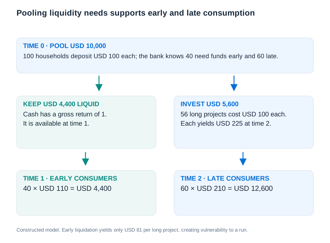
| Arrangement | Early consumption | Late consumption | Initial projects financed | Expected utility |
|---|---|---|---|---|
| Individual cash storage | USD 100 | USD 100 | 0 | 7.6000 |
| Individual project investment | USD 81 | USD 225 | 100, of which 40 liquidated | 9.0000 |
| Pooling without extra smoothing | USD 100 | USD 225 | 60, none liquidated | 9.4000 |
| Pooling with smoothing | USD 110 | USD 210 | 56, none liquidated | 9.4121 |
Financial intermediation does not always increase the number of projects initially financed. Here it reduces investment from 100 projects to 56 while increasing welfare. In direct investment, 40 projects are subsequently destroyed early; in the pooling arrangement, liquid resources are planned from the outset and consumption is better allocated across states. Investment volume alone is therefore not a sufficient measure of the bank’s contribution.
The resource constraint and the exact smoothing optimum
The USD 110/210 contract is a convenient feasible improvement, not the exact optimum. To derive the latter, let the bank hold enough cash for early payments and put everything else into projects. With 40 early and 60 late households, the budget is:
One extra dollar to each early household costs USD 40 in cash and forgoes USD 90 of mature project proceeds, reducing each of 60 late payments by USD 1.50. Maximising yields:
Solving both conditions gives , and expected utility approximately 9.412757. This assumes divisible projects and the stated preferences. Since , a late household prefers waiting to withdrawing and storing the money, provided other late households also wait. The tiny improvement over USD 110/210 explains why the rounded contract is useful without mislabelling it as the exact mathematical solution.
The economic framework originates in Diamond and Dybvig, Bank Runs, Deposit Insurance, and Liquidity (1983). The numerical model here is the specified 100-household illustration, with its feasibility and utility calculations shown explicitly.
The no-run equilibrium
Return to the USD 110/210 contract. A late household’s payoff depends on other households’ withdrawal decisions. If all other late households wait, the bank uses its USD 4,400 cash for the 40 early consumers and keeps all 56 projects until maturity. A particular late household, X, then receives USD 210 at date 2 and utility . If X instead withdraws at date 1, it receives USD 110, stores that amount until date 2 and obtains utility .
That extra withdrawal forces liquidation of projects once the normal cash buffer is exhausted. X still prefers waiting because USD 210 exceeds the USD 110 it could store. Since the same reasoning applies to every late depositor when the others wait, no early withdrawal by late consumers is a Nash equilibrium. A Nash equilibrium means no individual benefits from changing its action while all others keep theirs; it does not mean the outcome is guaranteed to occur.
The run equilibrium and the cost of being last
Now suppose X expects the other 59 late consumers to withdraw early together with the 40 genuinely early consumers. Those 99 withdrawals request dollars. Liquidating every project produces only dollars; including cash, total liquid resources are . The bank cannot honour the promised early amount to everyone even though its investments would have yielded enough to support the intended allocation if left intact.
If X waits, the 99 other customers exhaust all liquid resources and no projects remain, so X receives zero at date 2. If X joins the run, all 100 customers queue. Under sequential service the first 81 receive USD 110 each, consuming USD 8,910; the 82nd receives the remaining USD 26; the final 18 receive zero. Assuming each place is equally likely, X’s expected cash receipt is:
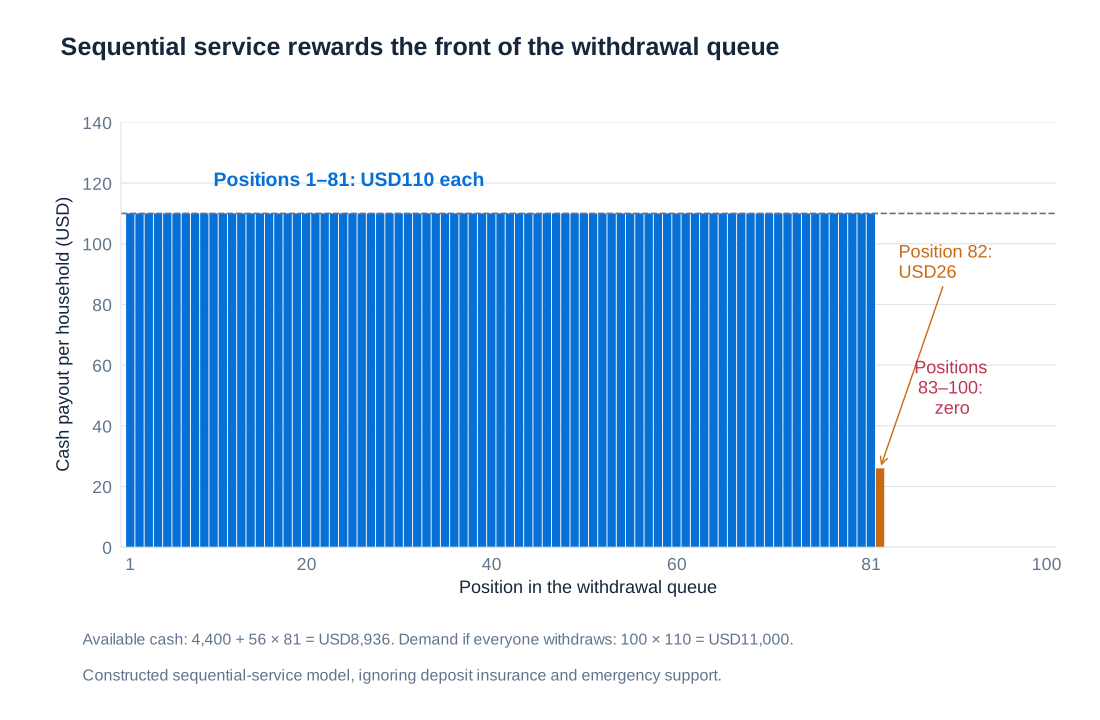
Because X is risk averse, expected utility must be calculated state by state. Applying utility to the average payout gives the wrong answer. The correct expected utility from running and storing the receipt is:
This is below , the utility of a certain USD 89.36, because the queue exposes X to payout risk. It nevertheless exceeds the zero utility from waiting when everyone else runs. Joining is therefore a best response, making the run another equilibrium. Individually rational actions can destroy collectively valuable liquidity insurance. “Panic” describes the adverse coordination outcome, not a proof that every depositor behaves irrationally.
The model isolates a run triggered by expectations without an initial deterioration in project fundamentals. In practice, runs can also reveal genuine insolvency, react to interest-rate losses or combine fundamental concerns with coordination effects. The distinction matters for intervention: providing liquidity to a viable bank and absorbing losses at an insolvent one solve different problems.
Deposit insurance, equal treatment and their limits
Suppose an external insurance scheme guarantees each depositor at least USD 100, with credible resources and timely payment. If X waits while everyone else runs, it receives USD 100 from the insurer rather than zero, giving utility 6. If X joins, the first 81 queue positions still receive USD 110; all other positions are topped up to USD 100. Expected utility from joining is then . Insurance greatly reduces the downside of waiting, but this particular principal-only guarantee does not eliminate the incentive to run, because it protects 100 while an early successful withdrawal pays 110.
A stronger guarantee or different contract can remove the first-mover advantage if waiting preserves at least the relevant insured entitlement and payment is sufficiently prompt. Credibility, coverage limits and access to funds matter as much as the announcement of insurance. Protection financed from outside the failing bank also changes the resource constraint: the insurer’s payment cannot be treated as cash the original bank created. By weakening creditors’ incentives to monitor risk, insurance can increase moral hazard, which is why capital requirements, supervision, risk-sensitive charges and resolution arrangements are relevant complements.
Alternatively, imagine that liquidation proceeds must be shared equally among all 100 depositors, independently of who sought early payment. Each receives dollars. X then obtains the same cash amount by joining or waiting, removing the advantage of a better queue position under that rule. It does not restore the USD 210 late payment or recover the productive value destroyed by liquidation. The result is indifference, not a strict proof that no run can occur. Actual legal equal treatment after closure also need not reverse payments already made before intervention.
Northern Rock and observable depositor behaviour
The Northern Rock queues in 2007 provide a visible illustration of these incentives. Customers’ concerns included whether other customers would withdraw, whether branch service would stop and whether being late would leave them without access to funds. Some described moving money as a prudent response to others’ actions rather than as panic. This resembles the model’s strategic complementarity: another depositor’s withdrawal can make one’s own withdrawal more attractive. The photograph is evidence of the historical event, while the numerical model is a constructed explanation of one mechanism.

The episode should not be reduced to a pure belief shock. A real bank’s wholesale funding, asset liquidity, public support and information about its condition also matter. Visible queues can amplify existing concerns; online communication and rapid transfers can now spread and implement withdrawal decisions much faster. Payment interruption can motivate even an insured customer to move funds, so withdrawal alone does not reveal that a customer expects an uninsured ultimate loss.
Demand deposits versus locked term funding: a worked choice
A customer with USD 100 can choose a demand account paying 10% annually or a two-year term deposit paying 20% annually. Interest compounds and is paid on withdrawal or maturity. The demand account pays USD 110 after one year or USD 121 after two. The term account pays USD 144 after two years and cannot be withdrawn early. Keep the same 40% early/60% late type probabilities and the same utilities. Assume the customer cannot borrow against or sell the term claim; an early consumer obtains no date-1 consumption from it and assigns no value to its later payoff.
The two expected utilities are:
The customer prefers the lower-interest demand account because its early availability is valuable. The term deposit would need terminal payoff satisfying . Thus dollars. If is the annually compounded rate on the two-year term deposit, then:
Intermediate rounding matters: replacing the exact demand utility with 8.16 before solving changes the reported payoff and rate. The enormous break-even rate is not a realistic market estimate. It results from an extreme assumption that an early household cannot use the locked wealth at all and cares exclusively about early consumption. The exercise isolates a general insight: liquidity services can make demand funding cheaper than otherwise comparable locked funding. Removing the borrowing or withdrawal restriction, changing the type probabilities, adding risk or account services would change the premium.
Market discipline: useful monitoring and destabilising withdrawal
Market discipline occurs when investors or creditors react to bank risk through required returns, funding quantities and contractual terms, thereby influencing management before losses occur. Callable deposits give a creditor an exit option. If risky behaviour threatens funding, managers may limit that behaviour ex ante. Uninsured short-term wholesale creditors, including interbank lenders and money-market funds, have stronger direct loss incentives to monitor than fully protected small depositors. Equity and long-term debt prices also contain information, even when those investors cannot withdraw at par.
Discipline is neither automatic nor costless. Monitoring requires information and expertise; some creditors may free-ride on others, rely on guarantees or react to misleading signals. Withdrawal can punish a weak bank but also force inefficient asset sales and spread stress. A model in which the credible threat of withdrawal induces safe behaviour can explain demandable debt, but it does not establish that real-world deposits are inherently risk-free. The same mechanism can discipline managers and create an unstable coordination game.
Pillar 3 of the Basel framework supports discipline through public disclosure, complementing minimum requirements and supervisory review. Useful information enables investors to compare exposures, capital and risk, but disclosure cannot make all investors equally informed or prevent every run. Deposit insurance and the removal of sequential priority reduce the private benefit from monitoring through withdrawal; prudential oversight then has a larger role in constraining risk.
Empirical work finds that deposit outflows depend on bank distress, uninsured exposure and the customer relationship. Brown, Guin and Morkoetter’s study of the 2007–09 crisis finds lower withdrawal risk among clients with strong pre-existing relationships and higher switching costs. The finding is about the studied setting, not a guarantee that relationship deposits never leave. Research by Jiang, Matvos, Piskorski and Seru links interest-rate-related asset-value losses and uninsured leverage to fragility in 2023. Work by Cookson and co-authors examines how social media can accelerate coordination. Motives may include loss avoidance, uninterrupted payment access, better interest rates or disapproval of the institution; observed withdrawals need not arise from a single motive.
Sources: Basel Pillar 3 disclosure framework; Brown, Guin and Morkoetter, Deposit withdrawals from distressed banks: Client relationships matter; Jiang and co-authors, Monetary Tightening and U.S. Bank Fragility in 2023; Cookson and co-authors, Social media as a bank run catalyst.
Modigliani–Miller as a benchmark for bank capital structure
A bank’s capital structure is the combination of debt and equity financing its assets. Under the frictionless Modigliani–Miller benchmark, changing that combination does not change total firm value if the underlying investment policy and total cash flows remain fixed. Perfect-market assumptions remove transaction costs, financing-dependent taxes, additional distress costs, information asymmetries and financing effects on investment. Debt can be risky in an extended version of the argument; what is excluded is an extra destruction of value merely from dividing the cash flows differently.
If a bank reduces leverage, its equity generally becomes less risky, so the return shareholders require can fall. It is therefore incorrect to multiply a fixed historical equity return by a higher equity share and infer that total financing costs must rise by that amount. The theorem provides a disciplined benchmark, not a literal description of banking: deposits provide services, guarantees create subsidies, taxes treat instruments differently and distress can destroy value. These departures explain why capital structure matters in practice. The classic cost-of-capital paper is from 1958; it should not be confused with the later dividend-policy work.


The trade-off theory and differences in asset risk
Trade-off theory balances benefits of debt, such as an interest tax shield where available, against expected costs of financial distress and related agency problems. Holding other factors constant, lower asset risk permits more debt for a given likelihood of distress. A bank’s diversified portfolio of cash, securities and senior loans can have lower measured asset volatility than the operating assets of a non-financial company. A loan is often a comparatively protected claim on a business, whereas the business’s own assets bear the full operating uncertainty.
This helps explain why banks often have greater leverage than non-financial firms; it does not establish that every bank has safer assets than every company. Concentrated lending, correlated defaults, market positions, duration exposure and off-balance-sheet commitments can all make a bank risky. Low volatility measured during normal periods may also conceal tail risk. Evidence on average differences in asset risk therefore supports a conditional explanation of leverage, not a blanket endorsement of a thin equity buffer.
Liquidity production and the special role of bank debt
Ordinary corporate debt primarily finances a firm. Bank deposits also produce services that customers value: payments, safekeeping and access to liquidity at short notice. Depositors may accept a lower yield in exchange for these services, creating a convenience benefit for the bank. Under liquidity-production theories, risk management helps the institution issue liabilities that users regard as safe and liquid. Replacing every deposit with ordinary equity would eliminate the deposit service, because an equity claim fluctuates in value and is not a promise to pay a fixed amount on demand.
That observation does not imply that any additional equity destroys liquidity creation. The bank can replace other debt, retain earnings or change its scale, and stronger capital can make deposits safer. The relevant question is the marginal effect of a financing change under explicit assumptions about assets, services, risk and regulation. Models in which high leverage supports liquidity production explain one force favouring debt; they do not by themselves identify the socially optimal capital ratio.
Discipline and the government safety net
A second bank-specific theory treats demandable short-term debt as a commitment device. Creditors can withdraw when they observe managerial diversion or risk taking, making misconduct costly to the bank. The threat can support prudent conduct in the model, provided monitoring and enforcement are effective. It is a theoretical explanation for why banks issue runnable debt even though runs are costly; the tension cannot be resolved by assuming the run threat has benefits but no possible costs.
A third explanation is the public safety net: deposit guarantees, access to central-bank liquidity and the expectation of extraordinary support can reduce creditors’ required compensation for risk. If the price of protection does not fully reflect risk, shareholders may prefer more leverage because part of the downside falls on the insurer, a resolution fund or ultimately the public. This creates a difference between privately attractive funding and socially desirable funding. It does not follow that every central-bank loan is a taxpayer subsidy or that every failed bank will be rescued: collateral, pricing, eligibility, loss allocation and resolution rules matter.
| Explanation | Mechanism | Implication and qualification |
|---|---|---|
| Modigliani–Miller benchmark | Financing only reallocates fixed cash flows | No value effect under its assumptions; real frictions must explain a difference |
| Trade-off theory | Debt benefits balanced against expected distress costs | Lower asset risk can support greater leverage |
| Liquidity production | Deposits supply valuable liquid claims | Some debt is an output of banking, but extra equity need not eliminate deposits |
| Market discipline | Withdrawal threats constrain managerial behaviour | Demandability can create incentives and also destructive runs |
| Safety-net incentives | Protection lowers private creditor exposure to loss | Private leverage can exceed the socially desirable level |
What empirical evidence can and cannot establish
Research comparing banks and non-banks finds that asset-risk differences explain a substantial part of their leverage difference. The remaining difference should not simply be labelled a precisely measured government subsidy: liquidity services, regulation, measurement and other institutional features can also matter. Likewise, evidence that historical capital ratios are weak predictors of crisis onset does not prove that leverage is harmless. Asset booms, funding composition, changes in asset risk and valuation losses can interact with the size of the loss-absorbing buffer.
The distinction between entering and recovering from a crisis is useful. Jordà, Richter, Schularick and Taylor’s historical work finds that better-capitalised banking systems recover more successfully after crises, even though high capital alone is not a reliable predictor of which systems will avoid one. A weakly capitalised bank suffering losses may cut lending or sell assets to restore a ratio, transmitting stress to borrowers. Capital absorbs losses and can support continued intermediation precisely when raising fresh equity is difficult.
Higher capital requirements can have short-run transition costs. Gropp, Mosk, Ongena and Wix’s analysis of the 2011 European capital exercise finds that affected banks increased ratios importantly by reducing risk-weighted assets and lending, with adverse effects on dependent firms. This identifies a response to a particular intervention, not a universal permanent effect of higher capital. Banks can also adjust through new equity, retained earnings or a different asset mix; timing and economic conditions influence which route they choose. A policy assessment must compare transition effects with the benefits of greater resilience and more stable lending over the cycle.
Empirical references include Berg and Gider (2017), What Explains the Difference in Leverage between Banks and Non-Banks?; Jordà, Richter, Schularick and Taylor, Bank Capital Redux: Solvency, Liquidity, and Crisis; and Gropp, Mosk, Ongena and Wix, Banks Response to Higher Capital Requirements. The mechanisms of liquidity production and demandable debt are developed respectively by DeAngelo and Stulz (2015) and Calomiris and Kahn (1991); the safety-net debate includes Admati and Hellwig (2013).
The funding decision therefore cannot be reduced to choosing the cheapest quoted interest rate. A bank must consider liquidity services promised to customers, the assets backing those promises, the incentives created by withdrawal rights and the losses its equity can absorb. A structure that is inexpensive in normal times can become costly when creditors demand cash simultaneously, while an adequate capital buffer and credible liquidity arrangements help preserve the services for which customers use the bank.
7. Banking Crises and Financial Instability
A banking crisis is more than a fall in bank share prices or the failure of a badly managed institution. It becomes systemic when distress threatens a substantial part of the financial system and disrupts its ability to provide payments, liquidity and credit. The same transformations that make banking useful create vulnerabilities: long-lived, risky and illiquid assets are financed with claims that customers expect to redeem promptly and at a predictable value. History therefore connects the organisation of banks with macroeconomic outcomes. The task is to identify the original shock, the mechanisms that amplify it and the policies that can restore intermediation without preserving unsustainable business models.
Five episodes illustrate different combinations of these mechanisms: the American savings-and-loan crisis; the Nordic crises; Japan's post-bubble banking problems; the global financial crisis of 2007–2009; and the interest-rate and property-market stress associated with the inflation and monetary-tightening cycle of 2022–2023. Their differences matter as much as their similarities. A duration loss, an insolvent borrower and a wholesale-funding run require different immediate responses, even though they can ultimately produce the same contraction in credit.
Identifying a systemic banking crisis
Laeven and Valencia's historical database identifies 151 systemic banking-crisis episodes worldwide during 1970–2017, including borderline cases. This is a count of country episodes, not a count of failed banks or independent global shocks. Several countries can enter crisis in the same international wave. Income classifications refer to countries' income at the start of each episode, using the World Bank's historical thresholds; classifying every observation by its present income would change the comparison.
The normal identification rule combines two conditions: substantial financial distress, evidenced by bank runs, banking losses or liquidations, and substantial policy intervention responding to that distress. The crisis starts in the first year when both conditions are met. There is an important severe-loss exception: very large observed losses or liquidations are sufficient even without three intervention measures. Specifically, the authors use non-performing loans above 20% of total loans, closures covering at least 20% of banking assets, or bank-restructuring fiscal costs exceeding 5% of GDP as indicators of sufficiently severe distress. These are research classification thresholds, not legal triggers for closing a bank.
| Intervention | Operational meaning in the historical database | Economic purpose and limitation |
|---|---|---|
| Deposit freeze or bank holiday | Restrictions on withdrawals, or temporary closure of banks | Interrupts a run, but also disrupts payments and access to savings |
| Significant nationalisation | Government takeover of a systemically important institution, including a majority equity stake | Permits restructuring and control; transfers governance responsibilities to the state |
| Bank restructuring expenditure | Gross fiscal restructuring costs of at least 3% of GDP | Restores loss-absorbing resources; gross expenditure differs from eventual net cost |
| Extensive liquidity support | Support exceeds 5% of deposits and liabilities to non-residents and more than doubles relative to its pre-crisis level | Relieves immediate refinancing pressure; cannot by itself repair negative economic equity |
| Significant guarantees | Broad government protection of liabilities, including protection extended to non-deposit bank liabilities | Restores confidence while creating contingent public exposure; a simple increase in deposit-insurance coverage does not qualify by itself |
| Significant asset purchases | Purchases by public authorities or their agencies exceeding 5% of GDP | Removes or funds troubled assets; the purchase price determines how losses are shared |
Normally, at least three of these six measures establish the intervention condition. The thresholds deliberately exclude minor failures and precautionary interventions that do not accompany systemic distress. However, the approach is not free from measurement difficulties: loss recognition can be delayed, non-performing-loan definitions differ, and a strong early response can reduce observed losses. Alternative databases use historical narratives, bank-equity price declines or credit and output contractions. A result about crisis frequency must therefore state which definition and observation period it uses.
Historical definitions, figures and comparisons in this section are from Laeven and Valencia, Systemic Banking Crises Revisited, IMF Working Paper 18/206 (2018). They describe 1970–2017 and do not constitute an inventory of subsequent banking events.
Crisis waves, currency pressure and sovereign debt
Banking crises occur in clusters rather than at a constant annual rate. The Latin American debt problems of the early 1980s, the transition from centrally planned economies, the Mexican crisis, the Asian crisis and the global financial crisis generated visible international waves. High-income economies were affected by the American savings-and-loan crisis, Nordic failures and Japan's crisis before 2007, but the global financial crisis greatly increased their representation in the dataset. The apparent calm of the mid-2000s was therefore poor evidence that severe banking instability had disappeared.
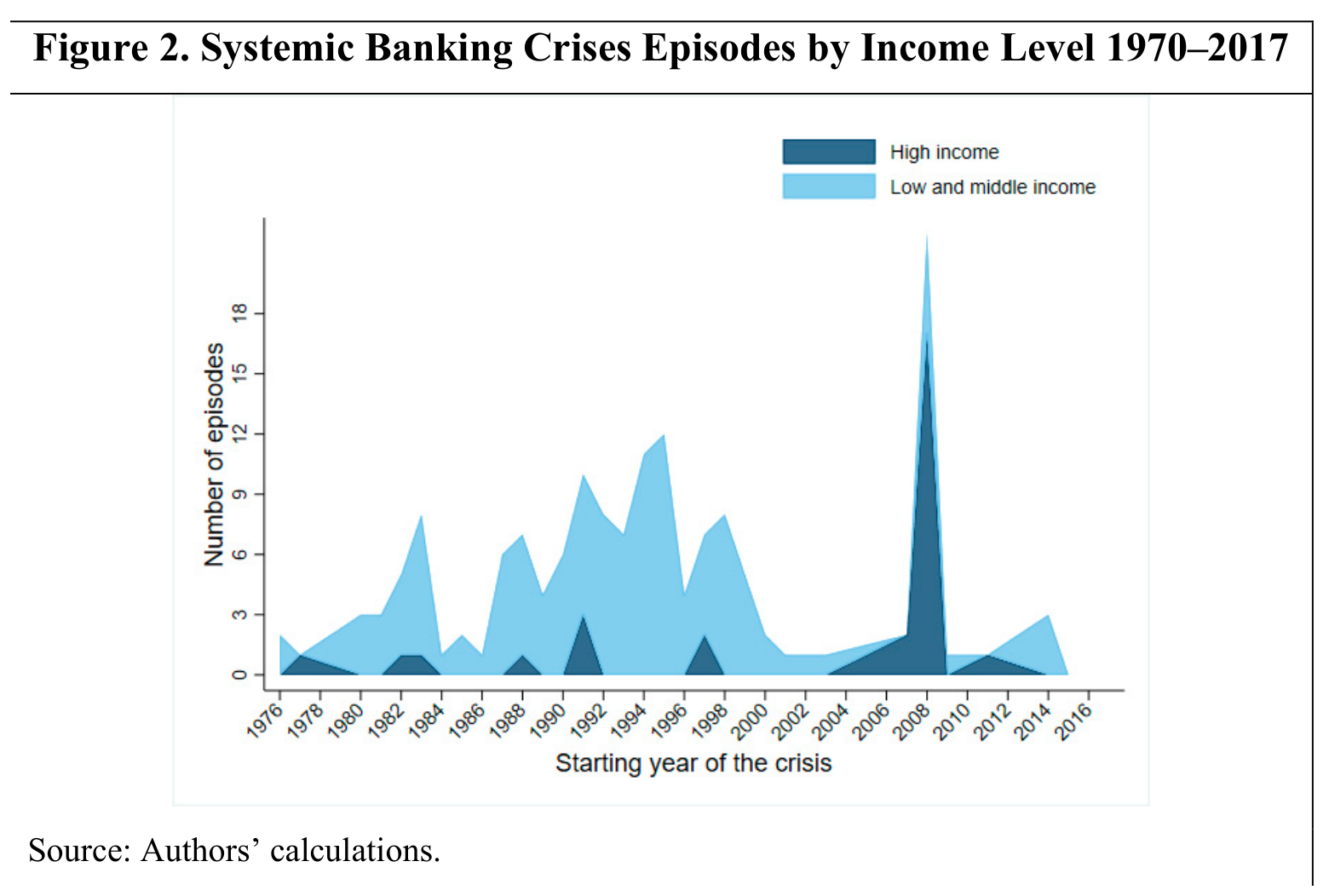
A currency crisis in this database requires a year-on-year depreciation against the US dollar of at least 30%, with the depreciation rate at least 10 percentage points higher than in the previous year. For repeated qualifying depreciations, the authors use the first year within a five-year window; early transition episodes are excluded. Sovereign-debt crises are dated using defaults to private creditors and/or restructurings. A twin crisis combines banking distress in year with a currency or sovereign crisis in ; a triple crisis includes both. These conventions prevent every exchange-rate movement or public-debt increase from being called a separate crisis.
| Banking-crisis category | Episodes | Share of banking episodes |
|---|---|---|
| Banking crisis without a currency or sovereign crisis in the overlap window | 107 | 70.9% |
| Banking and currency crisis, without sovereign crisis | 31 | 20.5% |
| Banking and sovereign crisis, without currency crisis | 2 | 1.3% |
| Banking, currency and sovereign crisis | 11 | 7.3% |
| All banking episodes | 151 | 100.0% |
The counts imply 107 standalone banking episodes and 44 overlapping episodes, so the overlapping share is . A country can experience banking distress without either of the other two crisis types. Nevertheless, the connections are powerful. A currency depreciation increases the domestic-currency burden of foreign-currency debt; bank rescues can weaken sovereign finances; and losses on sovereign bonds can impair banks that hold them. Depositors fleeing domestic banks may also move into foreign assets, adding exchange-rate pressure. In the historical sample, currency and debt crises tend to coincide with or follow banking crises, with currency episodes most frequent one year after banking distress begins. Temporal ordering alone does not prove that banking distress caused every subsequent event.
Containment, restructuring and the limits of liquidity support
Crisis containment tries to prevent a destructive interruption in payments and funding. Central-bank lending can replace suddenly unavailable private funding, while guarantees can convince creditors to maintain their claims. In the database, peak liquidity support is measured relative to deposits and liabilities to non-residents, rather than relative to GDP. Its median reaches 20.2% across the sample, approximately 12% for high-income economies and 23% for low- and middle-income economies. The increase above the pre-crisis level is a separate measure: its medians are 6.4% and 14.8%, respectively. A large pre-existing reliance on central-bank funds makes the distinction important.
Guarantees were announced in 34 episodes, including 19 in high-income countries. Their credibility depends on the state's fiscal capacity: promising more than the government can plausibly honour may transfer the panic from banks to the sovereign. Guarantees can also remain in force for years after immediate conditions improve. Deposit freezes and bank holidays are more disruptive and were rarer: the study records eight freezes and six bank holidays, with each recorded holiday followed by a freeze. A temporary closure can give authorities time to implement a restructuring, but it is not a way of making underlying losses disappear.
Resolution addresses the allocation of losses and the restoration or orderly withdrawal of banking services. Viable institutions may need new equity, changes in management and business-model repair. Institutions that cannot be made viable need an orderly transfer or wind-down. An asset-management company, often called a bad bank, can separate difficult assets from continuing banking operations and provide specialised recovery expertise. Separation works only if valuations are credible and someone bears the loss: selling a bad loan at an inflated price merely hides a public subsidy. Recapitalisation, asset transfers and nationalisation are distinct instruments, although they can be combined in the same programme.
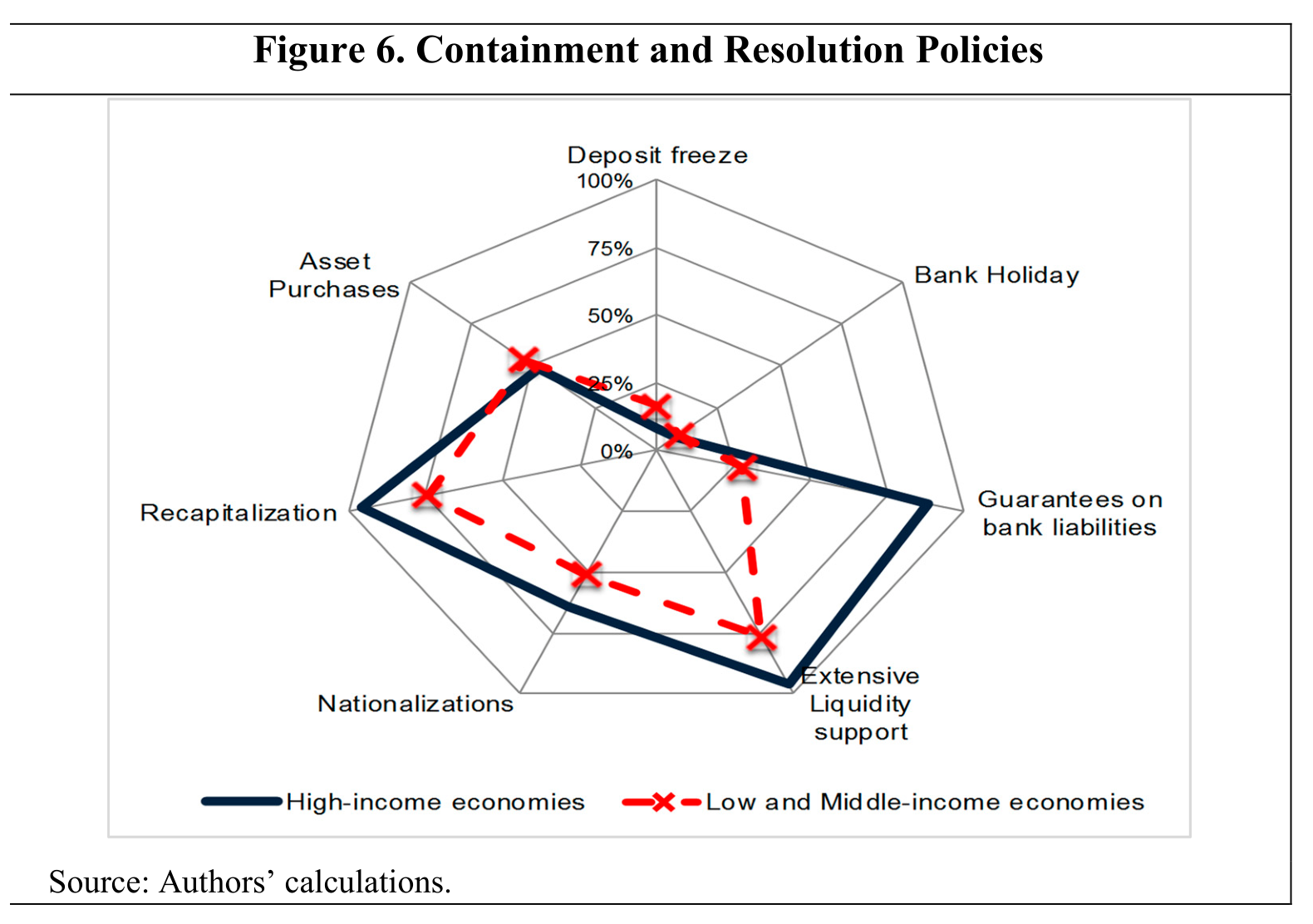
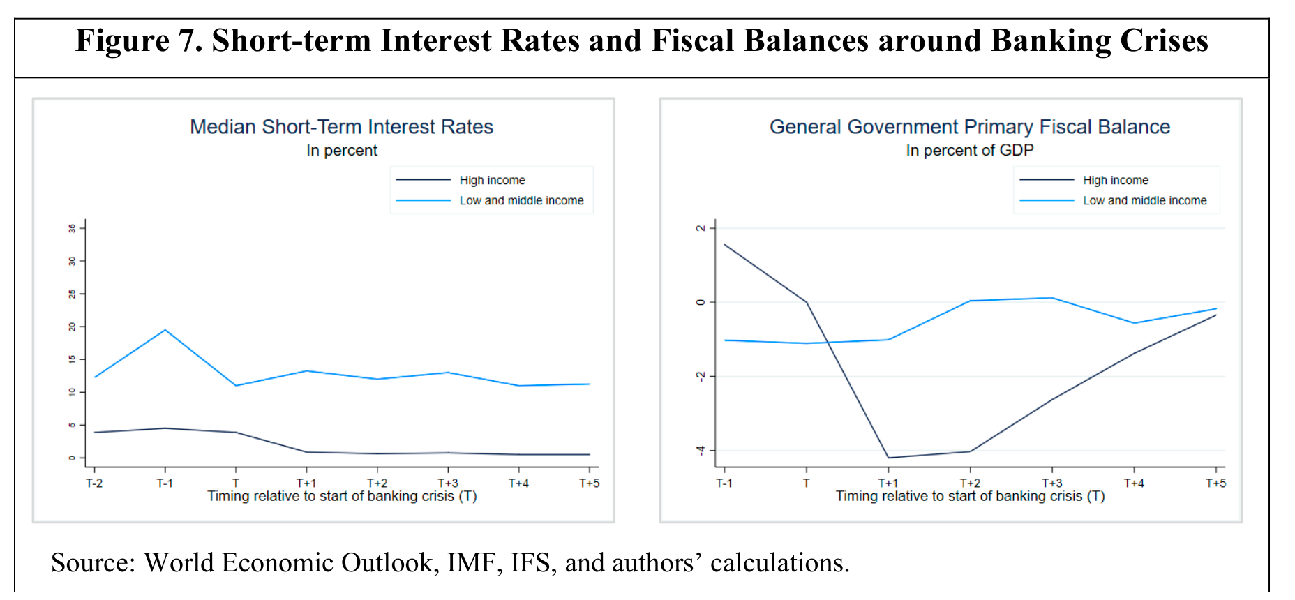
Macroeconomic policy also differs across countries. In high-income episodes, median short-term interest rates fell from around 5% towards zero after the onset of crisis, and primary fiscal balances deteriorated. Lower-income economies were more frequently constrained by currency pressure and access to public borrowing; interest rates could rise and fiscal policy become contractionary. These are historical associations rather than prescriptions. Cutting rates may support domestic demand but aggravate a foreign-currency mismatch if it triggers depreciation. A financial rescue should therefore be evaluated jointly with the monetary, fiscal and exchange-rate constraints under which it operates.
Fiscal expenditure, output loss and the length of recovery
Gross fiscal cost measures public outlays directly associated with financial-sector intervention: capital injections, administrative costs, payments on guarantees that are actually called and other rescue expenditure. An uncalled guarantee is contingent exposure, not an immediate cash expense. Net fiscal cost deducts recoveries such as proceeds from selling acquired assets, dividends, interest and guarantee fees. Unsold assets' unrealised gains are not equivalent to cash recoveries. The historical database divides each year's outlay by that year's nominal GDP and sums those ratios; values expressed relative to financial-system assets use a different denominator and answer a different question.
| Measure | High-income economies | Low- and middle-income economies |
|---|---|---|
| Gross direct fiscal cost, percentage of GDP | 6.7% | 10.0% |
| Net direct fiscal cost, percentage of GDP | 3.3% | 9.6% |
| Increase in public debt, percentage points of GDP | 21.1 | 16.4 |
| Peak non-performing loans, percentage of loans | Slightly above 11% | 30% |
| Duration pattern under the study's convention | More than half last five years or longer | Most last four years or less |
Gross and net medians use different available samples because recoveries are not observed for every episode. Their difference cannot be treated as the median recovery amount. Public-debt increases also include recession-related revenue losses, automatic stabilisers, fiscal stimulus, interest and GDP-denominator effects; they are broader than bank-rescue expenditure. For post-2007 episodes the study compares the change in debt with pre-crisis projections, whereas earlier episodes use the actual change. These distinctions explain why the high-income group can show lower direct rescue costs but a larger rise in public debt.
| Country and crisis start | Gross fiscal cost, % GDP | Net fiscal cost, % GDP | Cumulative output loss, % trend GDP |
|---|---|---|---|
| Finland, 1991 | 12.8 | 11.1 | 69.6 |
| Norway, 1991 | 2.7 | 0.6 | 5.1 |
| Sweden, 1991 | 3.6 | 0.2 | 32.9 |
| Japan, 1997 | 8.6 | 8.5 | 45.0 |
| United States, 2007 | 4.5 | 0.6 | 30.0 |
| Germany, 2008 | 2.7 | 0.7 | 12.3 |
These figures use the database's 2018 information set and measurement conventions. They show why a regional label such as “Nordic crisis” does not imply identical outcomes and why subsequent asset recoveries can materially reduce fiscal cost. The country-level database also records dates, NPLs and policy instruments; those are research observations rather than additional universal crisis rules.
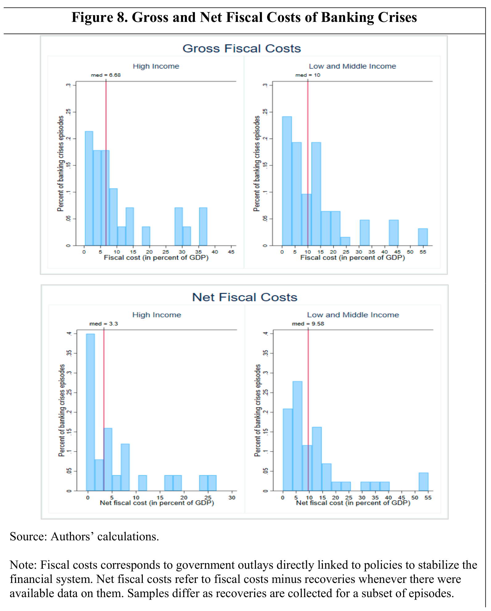
Output loss measures the cumulative shortfall of real GDP from an extrapolated pre-crisis trend during the crisis year and the following three years. The study estimates the trend using a Hodrick–Prescott filter with smoothing parameter 100 on pre-crisis log real GDP, normally using twenty years of history. The four-year cumulative shortfall is expressed relative to a year's trend output. A reported loss around 35% for high-income episodes does not mean that GDP necessarily fell by 35% in a single year: four gaps of roughly 9% would already produce a cumulative figure near that size.
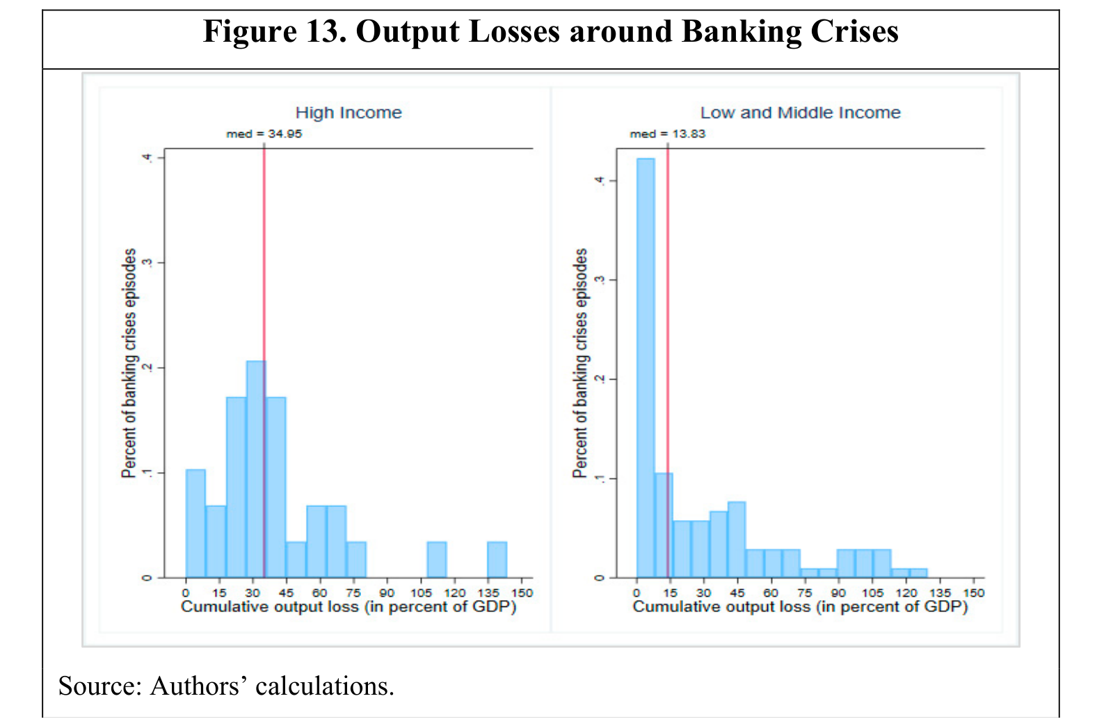
A simple constructed example clarifies the distinction. Suppose the no-crisis path is 100 units of GDP in each of four years and actual output is 94, 90, 91 and 95. The cumulative shortfall is units, or 30% of one year's benchmark output. If government rescue spending is 7 units and subsequent cash recoveries are 4, direct net fiscal cost is 3 units. The economy can therefore suffer a large production loss even when the eventual rescue bill is relatively modest. Neither calculation by itself isolates causation: an energy shock or global trade slump may contribute to the observed output gap.
The historical endpoint of a crisis is the year before real GDP and real credit growth are both positive for at least two consecutive years. When credit data are unavailable, the authors rely on GDP growth. Duration is capped at five years, so a recorded five-year episode means five years or longer, not necessarily full recovery after year five. Credit stocks can remain weak because of loan write-offs even when new lending has resumed. Moreover, positive growth can coexist with output permanently below its earlier path. The paper's output and export profiles show especially persistent shortfalls in high-income economies; many of those observations belong to the global financial crisis, when weak external demand limited recovery through exports.
The savings-and-loan crisis: maturity transformation and delayed recognition
American savings-and-loan associations traditionally financed long-term fixed-rate residential mortgages with shorter-term savings deposits. This business model was vulnerable when inflation and monetary tightening drove market interest rates sharply higher in the late 1970s and early 1980s. New deposit funding became expensive, while old mortgages continued earning low fixed rates. Even before borrowers defaulted, the present value of those mortgages fell. A thrift could consequently have positive historical-cost book capital while the market value of its assets was below its liabilities.
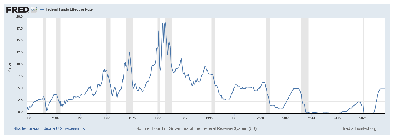
The shock interacted with deposit insurance, regulatory forbearance and deregulation. Allowing a weak institution to continue operating can create an incentive to gamble for recovery: shareholders retain the upside of a successful risky strategy while insured creditors and the public safety net bear much of the downside. Relaxed constraints and weak supervision enabled some institutions to expand into riskier activities instead of repairing their balance sheets. The episode was not simply an unavoidable consequence of high rates; institutional incentives affected the ultimate losses.
The crisis label “1988” in international datasets marks a systemic phase rather than the entire historical sequence. Troubles began earlier, and the Resolution Trust Corporation continued resolving thrifts until 1995. Estimates of outstanding assets, market-value losses and fiscal resolution costs should not be interchanged. The Federal Reserve's historical account reports 747 thrift closures by the RTC, with assets above USD 407 billion, and a taxpayer cost estimated as high as USD 124 billion. A claim that the crisis cost taxpayers USD 600–800 billion would therefore describe a different or inadequately specified quantity.
Two subsequent changes illustrate that risk can move rather than vanish. Adjustable-rate mortgages make the bank's interest income respond to funding rates, reducing some maturity mismatch, but the borrower may then become unable to afford higher payments: interest-rate risk becomes credit risk. Securitisation can transfer mortgages to investors, but weak originator incentives, guarantees and retained exposures may leave risk elsewhere in the banking or shadow-banking system. Risk management must follow the economic exposure through the transaction.
The historical chronology and fiscal-cost distinction are supported by Federal Reserve History, Savings and Loan Crisis, and the FDIC's historical studies of thrift resolution.
The Nordic crises: credit losses and transparent restructuring
Financial liberalisation and rapid lending growth contributed to property and credit booms in Norway, Sweden and Finland during the 1980s. When economic and property-market conditions deteriorated, loans that had appeared safe generated substantial losses. The central vulnerability was aggressive lending and weak asset quality, rather than maturity transformation alone. Loan-loss ratios rose from 0.7% of loans in Norway in 1987 to about 6% in 1991; from 0.3% in Sweden in 1989 to about 7% in 1992; and from 0.5% in Finland in 1989 to about 5% in 1992. These annual loss measures are different from the stock of non-performing loans.
Sweden became an influential example of restructuring because authorities recognised losses, guaranteed relevant bank liabilities, took control of severely distressed institutions and separated troubled assets into asset-management companies. Two large banks, Nordbanken and Gota, became central to the restructuring; their impaired assets were handled through Securum and Retriva. The viable banking operations could continue while specialists worked on asset recovery. Public protection of creditors did not require preserving the value of existing shareholders' investments.
The analytical lesson is the importance of credible recognition and incentives. Independent asset management, transparent valuations and a clear distinction between viable and non-viable institutions reduce pressure to keep bad loans alive. Private owners who can restore viability have an incentive to inject funds before losing control. However, the Nordic countries did not all experience identical policies, costs or recovery speeds. “The Nordic model” describes a family of approaches, and the Swedish institutional details should not be assigned indiscriminately to Norway or Finland.
Country loss ratios and resolution lessons are discussed in Federal Reserve Bank of St. Louis, Resolving a Banking Crisis, the Nordic Way (2009), and the European Commission's study of the Swedish banking-crisis response.
Japan: property collateral, evergreening and a prolonged adjustment
Japan's experience followed a long post-war period without major bank failures. Strong growth, low inflation and financial liberalisation supported optimistic expectations during the 1980s, while lending and collateral valuations became heavily exposed to real estate. The asset-price reversal around 1990 weakened borrowers and banks together. Land pledged as collateral no longer justified earlier loan amounts, and the recognition and disposal of problem loans proceeded slowly. The systemic crisis is dated 1997 in Laeven and Valencia, although important failures, public responses and recapitalisation continued into 1998 and beyond.
Evergreening means extending or renewing funding to a borrower whose underlying repayment capacity is inadequate, often to avoid recognising an existing loss. It differs from a commercially justified restructuring of a temporarily distressed but viable borrower. A bank with little capital may prefer to roll over a bad loan because recognising the loss would reveal that it needs recapitalisation. The strategy can protect reported ratios briefly while tying scarce credit and productive resources to weak firms. Competitors capable of using those resources more efficiently may then receive less finance.
A reported NPL ratio depends on the date, definition and institutions included. A late-1990s figure around 8% and the historical database's 35% peak for the Japanese episode are not reconciled measures with an identical date, definition and institutional perimeter. They should not be spliced into one consistent time series. The mechanism does not depend on choosing whichever statistic looks largest: delayed recognition, weak incentives and unresolved bank capital problems can prolong a credit impairment even when immediate runs are contained. The long period of weak growth often called Japan's lost decade had additional macroeconomic causes; bank distress and capital misallocation were important components rather than a complete explanation.
The global financial crisis: mortgage losses become wholesale runs
Before 2007, rising US house prices supported mortgage borrowing, refinancing and consumption. Prices approximately doubled in some widely used indices between 2000 and 2006, although the exact increase depends on the index and geography. When collateral keeps appreciating, refinancing can conceal weak repayment capacity; lenders and investors may extrapolate unusually favourable default experience. Securitisation broadened the supply of funding but also separated origination from ultimate loss bearing. Fees rewarded transaction volume, complex structures obscured risk, and short-term liabilities financed securities whose liquidity could disappear.
Potential contributing factors include global saving and capital flows, low financing costs, housing-policy incentives, weak underwriting, optimistic ratings, high leverage and the expectation of official support for important institutions. Their relative weight remains debated. It is too strong to explain the entire crisis by one policy or to assume that every mortgage securitisation is inherently defective. The decisive vulnerability was the interaction of common housing exposure with leverage, opacity and runnable finance.
| Period | Selected developments | Mechanism revealed |
|---|---|---|
| First half of 2007 | New Century Financial fails; Freddie Mac tightens its treatment of high-risk mortgages; mortgage and structured-credit losses become visible | Underwriting and valuation assumptions cease to hold |
| Second half of 2007 | IKB requires support involving KfW; asset-backed commercial paper funding contracts; Countrywide and Northern Rock face severe funding pressure | Investors refuse to roll over short-term claims against difficult-to-value assets |
| Early to mid-2008 | JPMorgan acquires Bear Stearns with Federal Reserve assistance; authorities expand liquidity facilities; IndyMac fails in July | Liquidity assistance and assisted transfers attempt to contain contagion |
| September 2008 | Fannie Mae and Freddie Mac enter conservatorship; Lehman Brothers files for bankruptcy; the Reserve Primary Fund breaks the buck; AIG receives emergency support; Washington Mutual fails | Counterparty fears and losses spread across banks, dealers, insurers and money-market funds |
| Late 2008 and thereafter | International interventions expand, including the original USD 700 billion TARP authorisation in the United States | Authorities move from isolated assistance towards system-wide stabilisation and recapitalisation |
Asset-backed commercial paper normally matures quickly. If investors refuse to buy replacement paper, the issuer must obtain alternative liquidity or sell the assets backing it. A run therefore need not involve customers queuing outside a branch. Money-market funds created a related vulnerability: investors expected a stable value and rapid redemption even when underlying securities were risky. After Lehman's failure, losses at the Reserve Primary Fund pushed its net asset value below USD 1 per share, encouraging redemptions and broader pressure on money-market finance. Early redemption can be attractive when later investors bear more of the cost of liquidating remaining assets.
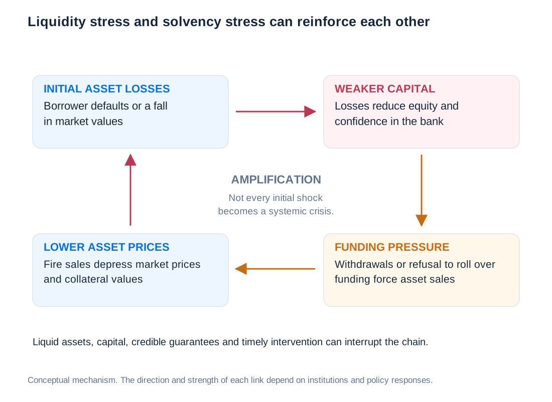
Fire sales connect liquidity and solvency. A sale depresses market prices, reducing collateral values and the measured capital of other holders; lenders demand higher haircuts or more margin; institutions sell further assets. An action that protects one institution can worsen system-wide outcomes. Bank runs are consequently powerful amplifiers, but many historical crises begin with deteriorating assets or unsustainable credit booms. Theoretical self-fulfilling runs remain possible: the historical tendency is not a theorem that panic can never be the initial cause.
The mortgage-credit mechanism and chronology can be compared with Federal Reserve History, Subprime Mortgage Crisis. TARP's original authorisation was a ceiling, not the same quantity as final expenditure or net fiscal loss.
Inflation, monetary tightening and bank fragility in 2022–2023
The rise in inflation and subsequent policy tightening exposed a different combination of weaknesses. Long-duration bonds and fixed-rate loans lost market value as discount rates increased. At the same time, real-estate borrowers faced more expensive refinancing and lower collateral valuations. Banks can be exposed through residential mortgages, direct lending to commercial-property companies and property collateral securing loans to other businesses. A government bond with very low default risk can still create substantial interest-rate risk.
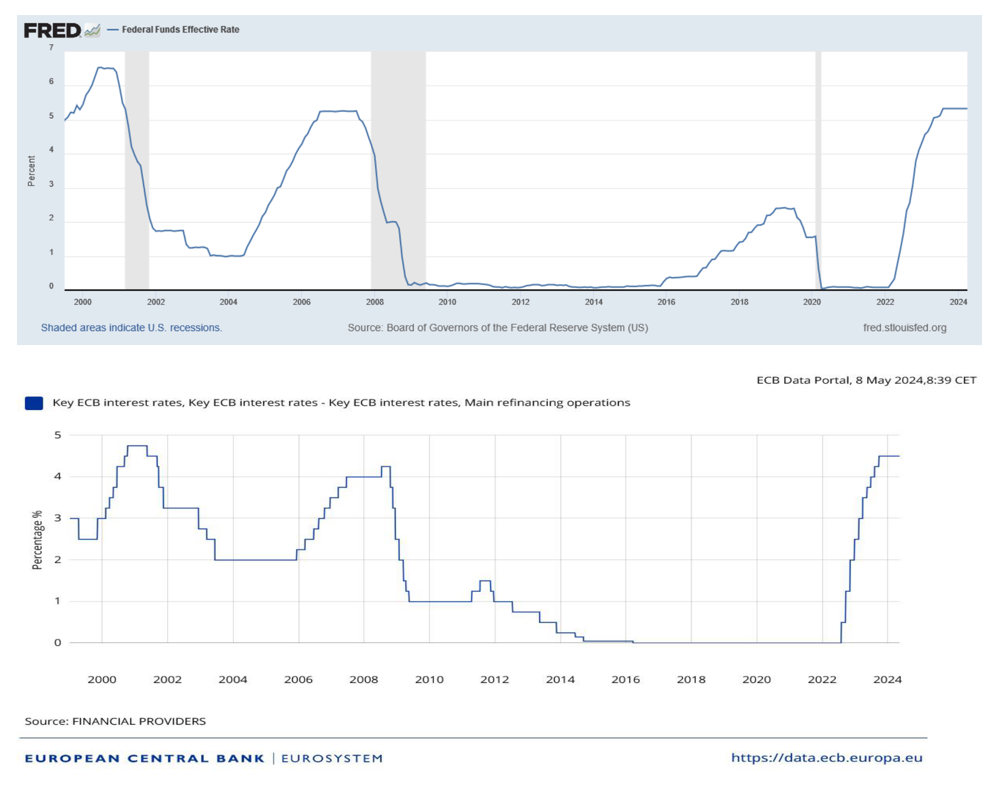
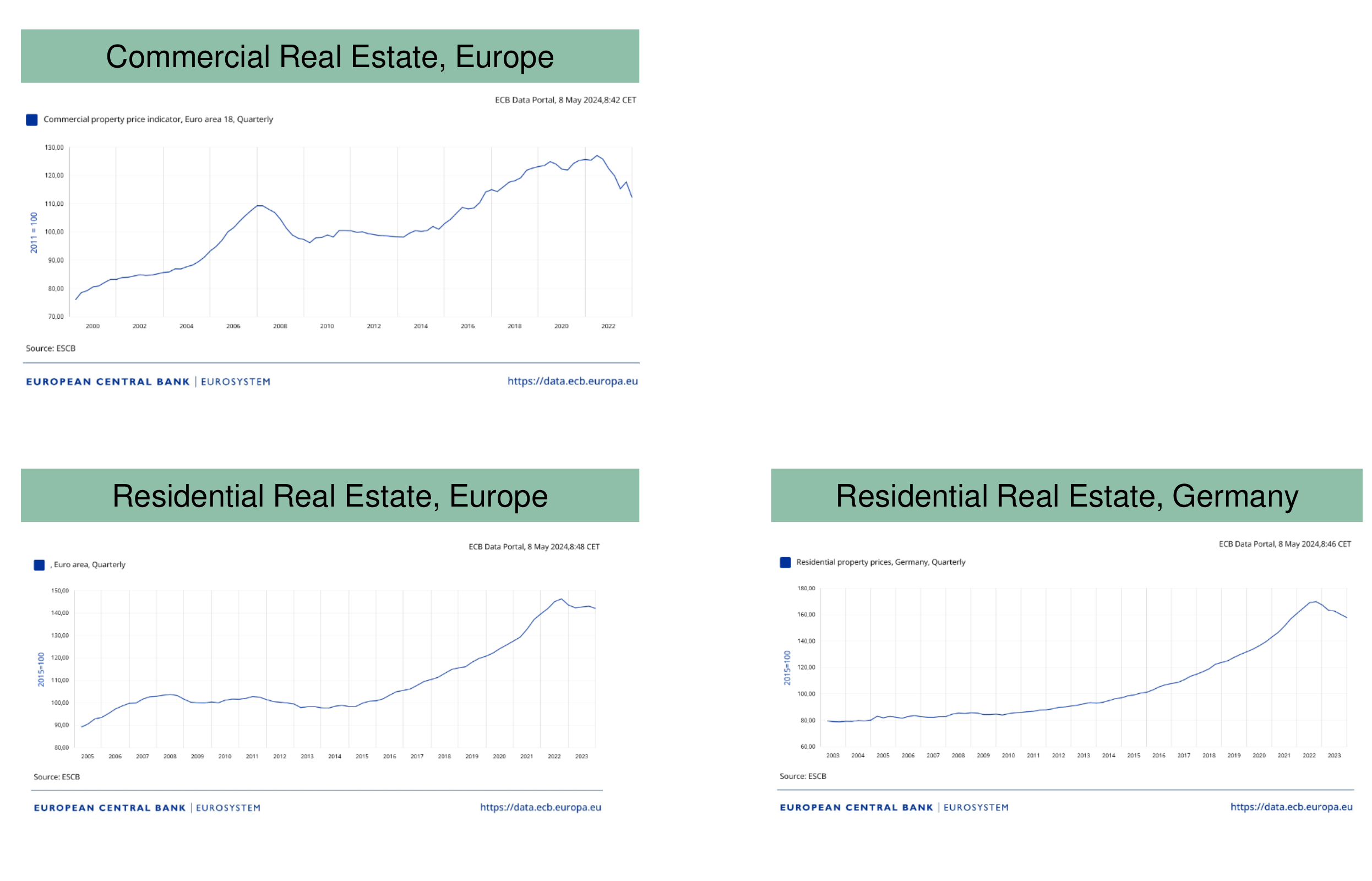
For a small parallel yield movement, modified duration provides the approximation
Here is the initial asset value, is modified duration in years, and is the yield change expressed as a decimal. A duration of five years and a two-percentage-point yield increase imply approximately . Convexity, non-parallel yield-curve movements, changing credit spreads and borrower prepayments can materially alter the result. The calculation concerns valuation, not an assumption that 10% of borrowers default.
Funding behaviour determines how that valuation loss affects the bank. Define the deposit beta as the change in the deposit interest rate divided by the change in the relevant market or policy rate. A beta below one means deposit remuneration rises more slowly, supporting the bank's margin and the economic value of its deposit franchise. However, this benefit depends on customers remaining with the bank. Depositors may move to higher-yielding alternatives or withdraw because they doubt the institution's strength. A scenario that marks assets to market and assumes immediate full pass-through to deposit rates is a demanding stress, not a complete going-concern valuation of every bank.
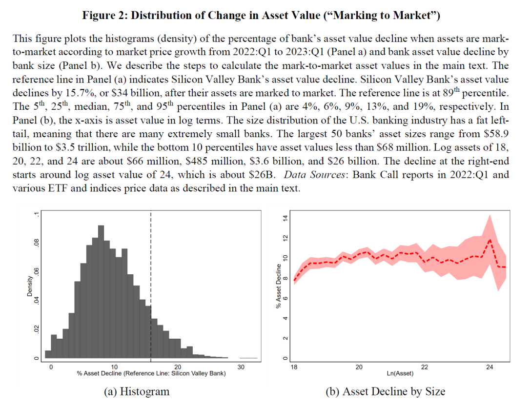
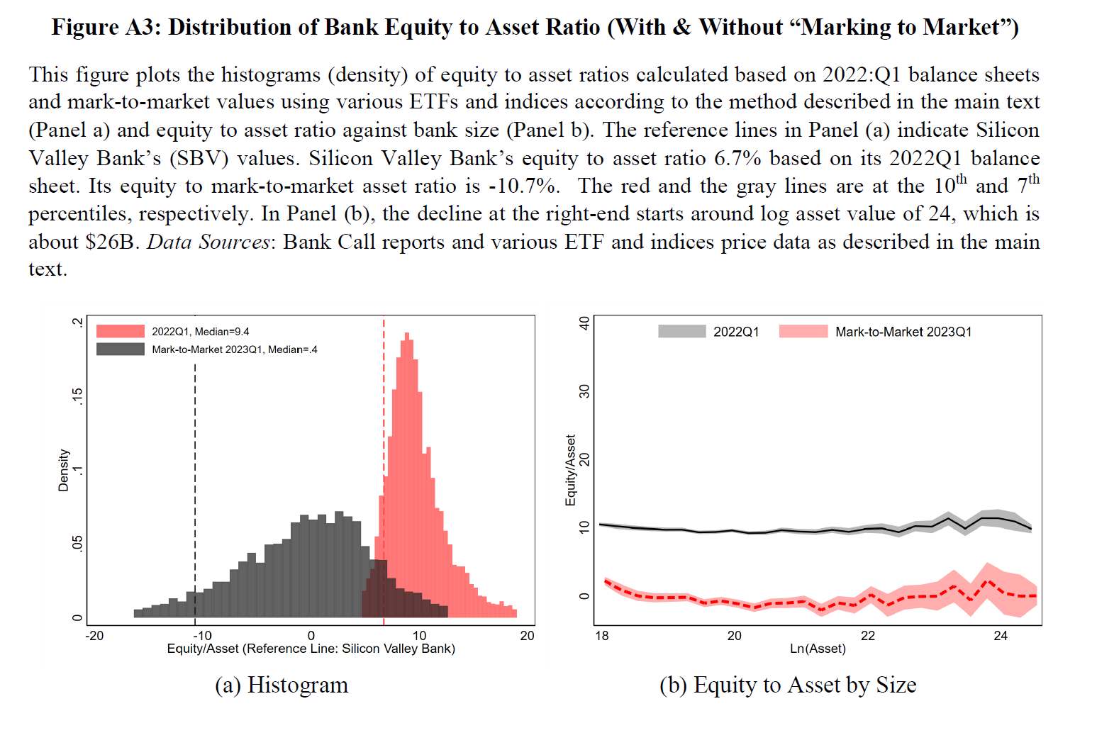
The 2023 analysis by Jiang, Matvos, Piskorski and Seru illustrates the scale of sensitivity when bank assets are revalued after monetary tightening. The distributions and bank-size comparisons identify vulnerability under stated assumptions; they do not mean that every institution with large unrealised losses must fail. Hedging, deposit stability, equity, cash buffers and access to collateralised liquidity matter. Conversely, historical-cost accounting does not guarantee that securities can be held to maturity if withdrawals require an immediate sale.
Silicon Valley Bank's March 2023 failure made this interaction concrete: concentrated uninsured deposits, rapid growth and inadequate management of interest-rate and liquidity risk left the bank exposed to a fast run. The Federal Reserve's April 2023 review also identified supervisory shortcomings. The case supports integrated analysis of assets, funding and governance. It does not establish that all banks with similar accounting losses had the same depositor behaviour or that interest-rate increases alone were sufficient to cause failure.
The bank-valuation figures retain the historical assumptions of Jiang, Matvos, Piskorski and Seru (2023), Monetary Tightening and U.S. Bank Fragility in 2023. The institution-specific account is supported by the Federal Reserve's review of Silicon Valley Bank.
Choosing a response that restores credit allocation
Across these cases, credit booms, collateral optimism and qualitative asset transformation recur. Real estate is especially prominent because exposures are large, assets are long-lived and credit can influence the very prices used to justify additional lending. Deregulation can facilitate valuable competition but also rapid expansion before risk management and supervision adapt. Cross-border funding can support investment and then reverse abruptly. The relevant question is not whether one instrument is always dangerous, but whether the system can bear a common shock without losing its essential functions.
Policy design should begin with credible diagnosis: recognise losses, distinguish viable from non-viable institutions and establish who bears the cost. Prompt recapitalisation and transparent restructuring can allow healthy borrowers to regain access to credit. Indefinite liquidity support for insolvent firms can instead sustain evergreening. Asset-management companies need expertise and independence, and guarantees need an exit strategy. Market-based finance may provide alternative funding when banks retrench, but securities markets themselves can freeze; a diversified system and adequately capitalised banks improve resilience without eliminating every risk.
The three most useful checks are consequently causal. Was the original weakness in duration, underwriting, funding structure or incentives? Which balance-sheet and market mechanisms amplified it? Did the response restore viable intermediation or postpone the recognition of losses? These questions distinguish the Nordic loan-loss episode from the savings-and-loan duration shock, identify wholesale runs during the global financial crisis, and explain why both capital and liquidity regulation are needed.
8. Banking Regulation and Prudential Supervision
Bank regulation must be justified by a problem that private contracts and market discipline do not adequately solve. The fact that a bank can make a bad loan is not sufficient: ordinary businesses also make poor decisions. Banking is distinctive because its liabilities support payments and liquidity, its borrowers depend on relationships that are difficult to replace, and its failure can damage institutions and people who did not choose its risks. Public safety nets reduce some dangers while creating new incentive problems. Prudential regulation attempts to contain those problems without removing the economically useful transformations performed by banks.
Four quantities must remain separate throughout the analysis: central-bank reserves, accounting equity, qualifying regulatory capital and high-quality liquid assets. Reserves are an asset used for settlement and monetary-policy implementation. Equity is a source of funding and a residual claim. Regulatory capital includes instruments and adjustments defined by prudential rules. Liquid assets provide resources that can be monetised during funding stress. A bank can have adequate capital but insufficient immediately available liquidity, or abundant liquidity but assets worth less than its liabilities.
Safety nets, externalities and the case for intervention
Deposit contracts supply valuable liquidity insurance, but their redeemability creates run risk. Deposit insurance and central-bank liquidity reduce the incentive to withdraw merely because others might do so. At the same time, protection can weaken creditors' incentives to monitor the bank: an insured depositor may demand little compensation for a riskier loan portfolio. Shareholders retain the upside of risky strategies while part of the downside falls on an insurance fund or the state. This moral-hazard channel can encourage greater leverage, lower liquid-asset holdings and riskier lending. Capital and liquidity requirements constrain the resulting choices; supervision and risk-sensitive insurance pricing can complement them.
A second argument concerns institutions whose disorderly failure would impose exceptionally large costs. A large bank may be difficult to resolve because it operates critical payment functions, has complex cross-border exposures or finances borrowers that cannot easily find substitutes. An expectation that authorities will rescue it can reduce its funding cost and reinforce risk-taking. This is the too-big-to-fail problem. The relevant characteristics extend beyond size to interconnectedness, complexity and substitutability.
Systemic risk also arises when many individually small institutions share the same exposures or funding structure. Each may rationally lend against rising property collateral, then sell the same assets during stress. Their combined actions can deepen the decline in collateral values and credit supply. Regulation therefore needs a microprudential perspective on individual safety and a macroprudential perspective on common exposures, feedback loops and aggregate credit conditions. A system composed of small banks is not automatically safe.
| Objective | Problem addressed | Representative instrument |
|---|---|---|
| Safety and soundness | Insufficient loss absorption or unstable funding, including incentives created by the safety net | Capital, liquidity and governance requirements |
| Systemic stability | Contagion, shared exposures, fire sales and disruption of critical functions | Systemic buffers, countercyclical tools, recovery and resolution planning |
| Consumer and investor protection | Complexity, information asymmetry, conflicts of interest and unsuitable products | Disclosure, suitability, conduct and complaints rules |
| Competition and access | Market power, barriers to entry and discrimination | Competition policy, proportionate authorisation and access rules |
| Financial integrity | Money laundering, fraud, sanctions evasion and terrorist financing | Customer due diligence, monitoring, reporting and internal controls |
| Monetary-policy implementation | Management of settlement liquidity and short-term money-market conditions | Reserve requirements, central-bank facilities and market operations |
| Specific credit-allocation goals | Public-policy objectives not supplied by unassisted markets | Targeted programmes, guarantees or lending restrictions, assessed separately from prudential safety |
Consumer protection is distinct from solvency regulation. Financial contracts can be difficult to assess even after purchase: a good outcome may reflect luck, while a poor outcome may reflect an appropriately disclosed risk. Customers cannot always reverse a mortgage or investment transaction as they would return an ordinary product. Transparency, product governance and fair advice address these frictions. Banks also serve as practical points for enforcing financial-crime laws because they observe accounts and payment flows. Compliance failures can generate fines, legal exposure and damage to confidence, as illustrated by the Danske Bank money-laundering and BNP Paribas sanctions cases; financial integrity is not a substitute for credit-risk control.
The intensity and type of rules should follow activities. Brokerage and payment infrastructure primarily raise conduct, operational and financial-integrity issues, although their scale can also be systemic. Institutions that perform qualitative asset transformation require particular attention to solvency and funding. The same functional reasoning applies to FinTech and non-bank intermediaries: a new technological label does not eliminate a familiar maturity or liquidity mismatch. Conversely, imposing a deposit-taking bank's entire rulebook on a business that does not bear those risks can create unnecessary costs.
Why bank capital matters for firms and employment
When loan losses erode bank equity, a bank can raise fresh capital, retain earnings, sell assets or reduce lending. New equity is often hardest to obtain precisely when investors doubt asset valuations. A weak bank may therefore restrict even profitable lending to restore its ratios. The resulting credit contraction harms borrowers that cannot easily replace a lender, particularly when the incumbent bank holds private information obtained through years of monitoring. A solvent small firm can experience financial distress because its bank is weak.
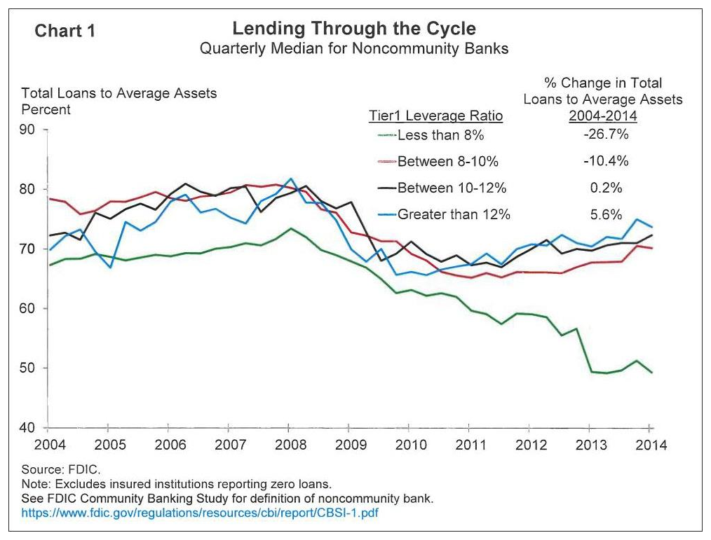
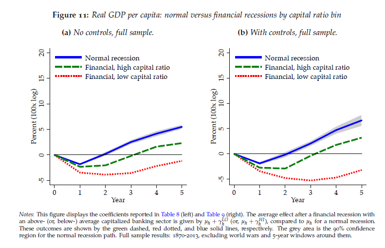
Historical comparisons associate stronger pre-crisis bank capital with more resilient lending and recovery, but a chart grouping banks by capital does not on its own establish causation. Better-capitalised institutions can also differ in management, loan composition and customers. More informative research designs try to distinguish bank credit-supply shocks from reduced borrower demand.
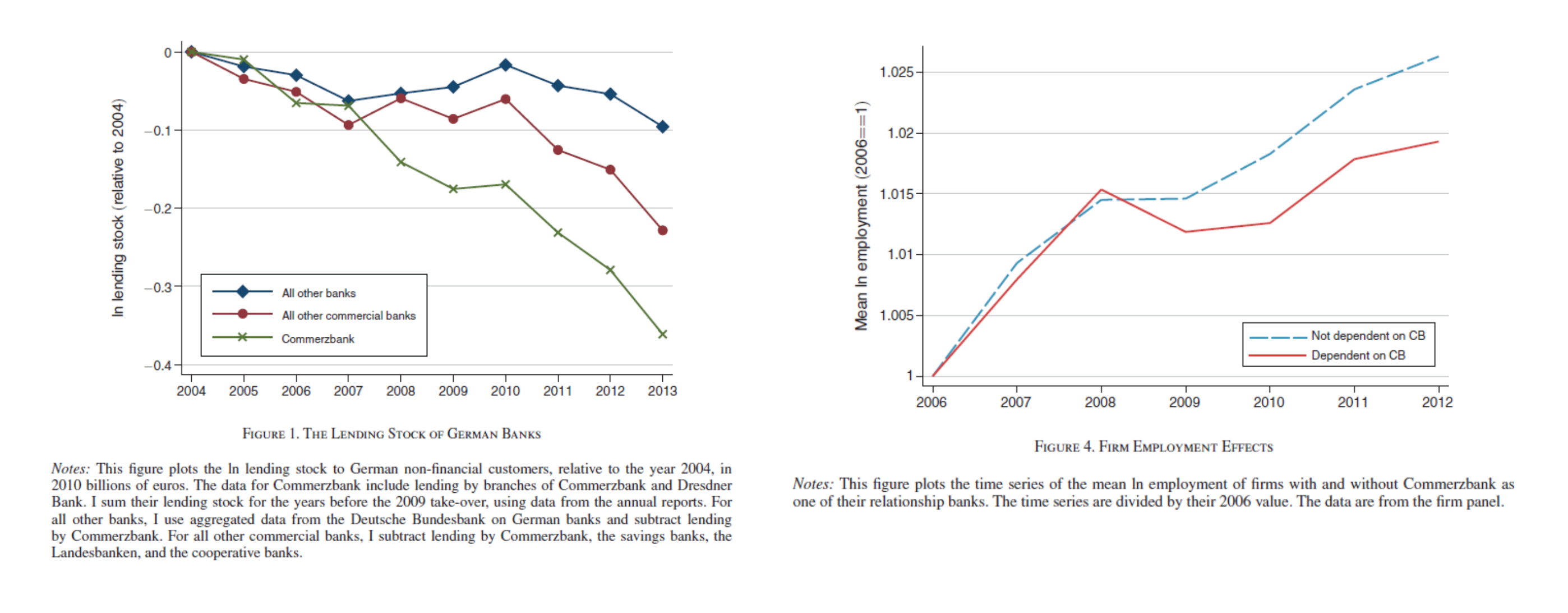
Huber's study of German firms and counties examines the effects of Commerzbank's lending reduction after its 2008 losses. Firms more dependent on the affected bank performed worse, and the effects extended to local economic activity. Existing relationships were not costlessly replaceable because potential new lenders lacked the incumbent's information. The evidence supports a real-economy cost of bank distress; it should not be interpreted as a claim that every exposed firm was categorically unable to obtain any alternative loan. Preserving bank resilience before a shock can protect productive activity beyond the bank itself.
Minimum reserves: a monetary asset requirement
In the Eurosystem, institutions subject to reserve requirements hold qualifying balances at their national central bank. The requirement is calculated on a defined reserve base, not on total accounting assets. Under the framework described by the ECB and Bundesbank, the positive ratio is 1%, principally covering overnight deposits, deposits with maturity or notice of up to two years and debt securities with maturity up to two years. Specified longer-term liabilities and repos have a zero ratio, while liabilities to the Eurosystem and other institutions subject to the reserve system are excluded under the rules. Each institution deducts a EUR 100,000 allowance from its calculated requirement.
Compliance is assessed using the average daily closing balance during a maintenance period. This averaging lets a bank accommodate day-to-day payment fluctuations while still satisfying its overall obligation. Minimum required reserves have been remunerated at 0% since September 2023. The rate paid on other central-bank holdings depends on the facility and applicable rules; it should not be inferred from the remuneration of required reserves.
For a simplified qualifying reserve base of EUR 1 billion, a 1% ratio gives EUR 10 million before the allowance and EUR 9.9 million after it. The calculation illustrates an asset-holding requirement. It does not mean that the remaining EUR 990.1 million can automatically be lent, nor that a bank must first receive reserves equal to the full principal of every new loan. Funding, settlement, capital and liquidity constraints interact, as the monetary chapter explains. Reserve settings are monetary-policy parameters and can be changed; they should be checked separately from prudential capital ratios.
The reserve base, averaging and allowance are described by the Bundesbank. The ECB provides the reserve framework and its decision on minimum-reserve remuneration.
Capital is funding that can absorb losses
A capital requirement does not normally instruct a bank to place shareholders' money in an unusable cash box. It determines how much qualifying loss-absorbing funding must support the bank's exposures. If shareholders contribute EUR 10 million, the bank can use the cash to make loans or acquire securities; the equity claim remains on the funding side while the asset composition changes. If a loan subsequently loses value, equity absorbs the loss before ordinary senior creditors. The requirement concerns the liability and ownership structure, while liquidity requirements concern assets and cash-flow resilience.
Regulatory capital differs from accounting equity because prudential rules specify eligible instruments and deductions. Common Equity Tier 1, or CET1, includes qualifying common shares and retained earnings after relevant adjustments and is the highest-quality component. Additional Tier 1, or AT1, comprises qualifying perpetual instruments with discretionary distributions and contractual loss-absorption features. Tier 1 is CET1 plus AT1 and supports going-concern loss absorption. Tier 2 includes qualifying subordinated instruments with specified eligibility and maturity conditions, contributing to loss absorption at non-viability or resolution. The labels do not mean that every instrument called “hybrid” or “subordinated debt” automatically qualifies.
Capital serves both a buffer and an incentive function. More equity allows a given loss to occur without making creditors bear it; it also makes shareholders bear a larger portion of the downside of risky decisions. There are trade-offs: rapid adjustment to a higher requirement can induce asset reduction, while a permanently stronger funding structure can lower fragility and support lending through a crisis. Comparing financing costs should consider the risk borne by each investor and any public subsidy to debt, rather than treating the observed equity return as a fixed cost independent of leverage.
Risk-weighted assets and a complete capital calculation
For a simple portfolio of on-balance-sheet credit exposures, risk-weighted assets are
is the regulatory exposure value, its applicable risk weight, the relevant category of qualifying capital and the corresponding ratio. In an actual return, exposure values can differ from accounting balances; collateral, guarantees, credit-conversion factors and netting may matter, while market, operational and other risks add to the aggregate risk exposure amount. A single credit-risk calculation should not be mistaken for the bank's complete legal requirement.
Consider the following historical teaching assumptions, in EUR million. They use a simplified pre-CRR3 risk-weight schedule to explain the arithmetic. In particular, the uniform 35% mortgage weight is not a statement of the current treatment of every residential mortgage: modern standardised rules depend on characteristics including loan-to-value, repayment dependence on property income and eligibility conditions.
| Asset | Exposure | Assumed weight | Risk-weighted exposure |
|---|---|---|---|
| Central-bank reserves | 20 | 0% | 0 |
| AA+ rated government bonds | 40 | 0% | 0 |
| A rated corporate loans | 430 | 50% | 215 |
| Qualifying residential mortgages under the assumed schedule | 600 | 35% | 210 |
| Total | 1,090 | Exposure-weighted average: 38.99% | 425 |
The funding is EUR 1,000 million of deposits plus EUR 90 million of equity, matching assets of EUR 1,090 million. The accounting equity-to-assets ratio is . Under the simplified assumption that all EUR 90 million qualifies as the relevant capital numerator and that no other risks or adjustments enter, , giving a risk-based ratio of . The two ratios describe the same bank using different denominators; the higher percentage does not create extra equity.
| Borrower category | AAA to AA− | A+ to A− | BBB+ to BBB− | BB+ to BB− | B+ to B− | Below B− | Unrated |
|---|---|---|---|---|---|---|---|
| Sovereigns | 0 | 20 | 50 | 100 | 100 | 150 | 100 |
| Banks | 20 | 50 | 50 | 100 | 100 | 150 | 50 |
| Corporates | 20 | 50 | 100 | 100 | 150 | 150 | 100 |
Other assumptions in this historical schedule are 0% for cash and central-bank balances, 75% for qualifying retail exposures, 35% for qualifying residential property, 100% for commercial property and other assets, and 100–150% for overdue loans. These categories are deliberately retained as a dated numerical exercise, not a current regulatory lookup table. Actual classification requires the jurisdiction's current law, due-diligence requirements and applicable approach.
A loan loss, the capital cushion and the denominator
Another bank has EUR 300 million of exposures weighted at 100% and EUR 200 million weighted at 50%, with EUR 44 million of CET1. Its simplified RWA is million and its CET1 ratio is . If a EUR 8 million loss reduces qualifying CET1 and RWA is held constant to isolate the numerator effect, capital falls to EUR 36 million and the ratio becomes .
Suppose, purely illustratively, its applicable CET1 hurdle is 10%. Before the loss it requires EUR 40 million and has EUR 4 million of headroom. Afterwards it is EUR 4 million short. If fresh eligible CET1 can be raised without increasing RWA, EUR 4 million restores the ratio. Alternatively, with capital fixed at EUR 36 million, it must reduce RWA to million, a reduction of EUR 40 million. A bank choosing the latter route by restricting lending can transmit its capital shock to borrowers.
The fixed-denominator assumption is useful but artificial. Writing down a 100%-weighted exposure may reduce both CET1 and RWA, while a downgrade can increase risk weights elsewhere; tax effects and prudential deductions can alter the numerator. Headroom also depends on which requirement is binding. A bank above its basic minimum may still fall into a buffer range, face distribution restrictions or breach a bank-specific requirement. “Above 8%” is therefore not a sufficient test of compliance.
From Basel I to the three-pillar framework
The Basel Committee's 1988 capital accord created an internationally coordinated minimum total capital ratio of 8% of RWA, including a 4% Tier 1 component. The broad risk buckets were simple and comparable but could treat quite different borrowers similarly. Historical national implementations included weights such as 0%, 10%, 20%, 50% and 100% for different categories; the precise classification varied. It is especially important to distinguish an asset risk weight from a credit-conversion factor that turns an off-balance-sheet commitment into an exposure before weighting it.
Basel II, published in 2004, increased risk sensitivity and organised the framework into three pillars. Pillar 1 sets minimum requirements for defined risks. Pillar 2 combines the bank's internal assessment with supervisory review, including risks incompletely captured by standard formulas. Pillar 3 requires disclosures intended to support market discipline. Internal-ratings-based approaches permit approved models to influence credit-risk calculations under supervisory constraints; external ratings and standardised categories play a different role in the standardised approach.
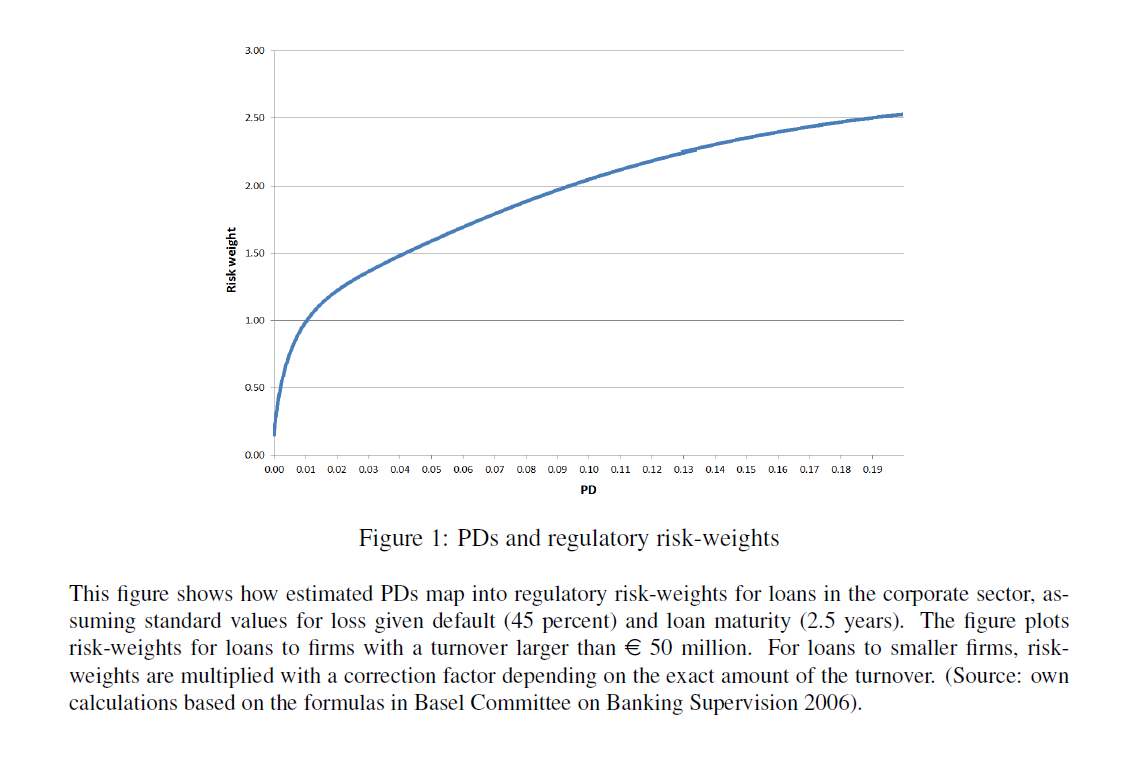
The historical corporate-risk-weight curve assumes a 45% loss given default, a 2.5-year maturity and borrower turnover above EUR 50 million; the horizontal variable is probability of default and the vertical variable is the risk weight. For smaller firms, the original model includes a turnover-dependent adjustment. The increasing curve explains why an estimated decline in PD can reduce required capital even when exposure volume does not change.
Model-based rules can recognise genuine differences in risk, but model outputs are not objective facts independent of incentives. A bank close to its capital constraint may have a strong incentive to obtain low estimated risk weights. Supervisors must assess data, estimation, validation and use, rather than assume that sophistication guarantees accuracy. Empirical work on model-based regulation has compared internal estimates and outcomes to study whether reported risk falls without a corresponding improvement in realised credit performance.
Mariathasan and Merrouche's 2014 study, The manipulation of Basel risk-weights, examines 115 banks in 21 OECD countries eventually approved to use internal ratings. Risk-weight density fell after approval, with a particularly pronounced decline among weakly capitalised banks and in weaker supervisory environments. Their evidence suggests strategic modelling contributes to the change; it does not imply that every reduction in a model-based risk weight is manipulation. This distinction is why both model validation and a less model-sensitive backstop are useful.
The global financial crisis exposed inadequate capital, opaque exposures and off-balance-sheet commitments, alongside funding fragility. It also revealed procyclicality: favourable market data lower measured risks during booms, enabling expansion, while defaults and volatility push requirements upward during recessions. Basel III responded with stronger capital quality and levels, buffers, a leverage backstop and explicit liquidity standards. These reforms complement rather than abolish the three-pillar structure.
Basel III minima, buffers and supervisory requirements
The basic risk-based Basel III minima are 4.5% CET1, 6% Tier 1 and 8% total capital, each measured against RWA. These are nested requirements, not percentages to add together. A bank can meet the additional Tier 1 and total-capital portions with higher-quality capital: it is not obliged to issue exactly 1.5% AT1 and 2% Tier 2. The capital conservation buffer adds 2.5% of RWA in CET1 above the minima, producing a baseline total-capital-plus-conservation level of 10.5% before other buffers or supervisory additions.
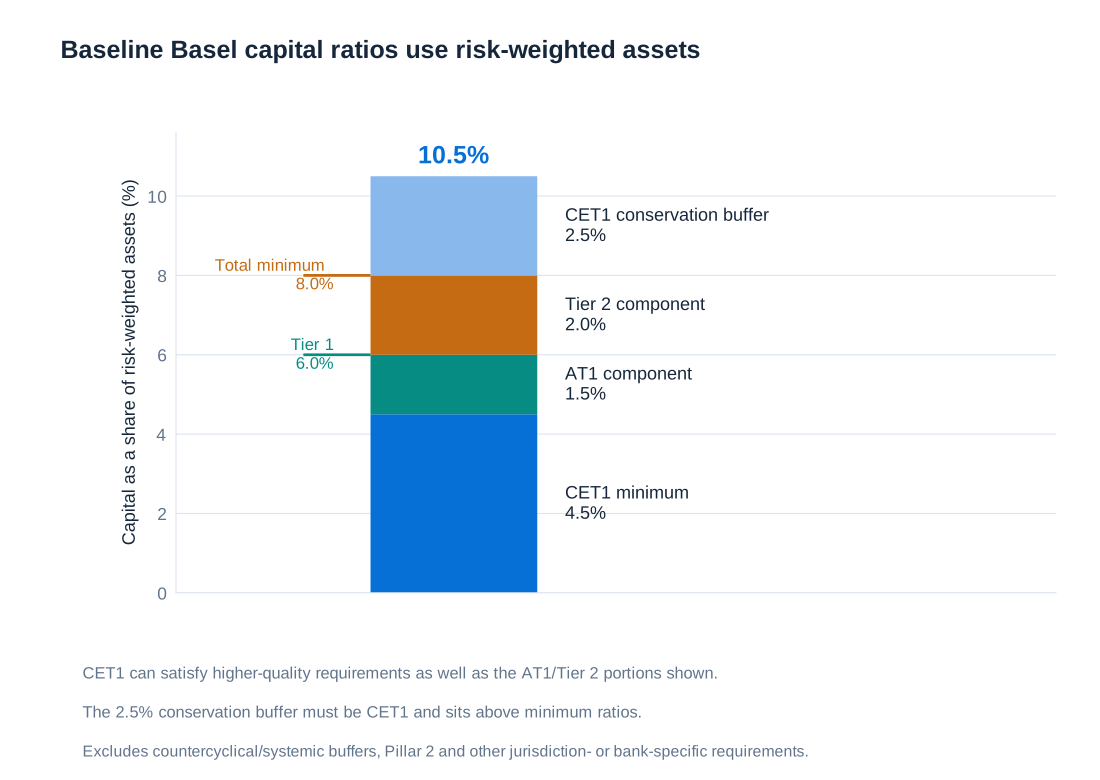
The conservation buffer is designed to be usable during stress. Falling into it activates restrictions on distributions, such as dividends and certain remuneration, rather than being identical to breaching the basic Pillar 1 minimum. The countercyclical capital buffer builds resilience as cyclical systemic risk accumulates and can be released when risk materialises, reducing pressure for an abrupt credit contraction. Raising this buffer simply because a crisis has already damaged bank capital would work against that intended release mechanism.
Global and other systemically important institutions can face additional buffers reflecting the costs of their failure. Systemic-risk buffers address defined structural or sectoral systemic risks under the applicable law. Their interaction and permitted combination depend on the legal framework: an old diagram showing the maximum of several buffers is not a universal current stacking rule. Bank-specific Pillar 2 requirements are binding, while Pillar 2 guidance expresses a supervisory expectation above binding requirements. A bank's own management buffer is a further business choice. Quoting one “normal” CET1 requirement for every European bank conceals these differences.
As an illustrative CET1 stack, take the 4.5% Pillar 1 minimum, 2.5% conservation buffer, a 1% institution-specific countercyclical buffer, a 1% systemic buffer and an assumed 1.125% CET1 component of Pillar 2 requirements. The resulting CET1 threshold is , before guidance and any voluntary headroom. The 1.125% arises if a 2% total Pillar 2 requirement has the standard minimum CET1 share of 56.25%; supervisors can require a higher-quality composition. These inputs are hypothetical and do not describe any named bank.
The minima and conservation buffer follow the Basel risk-based capital framework. The ECB distinguishes Pillar 2 requirements from Pillar 2 guidance.
Leverage, model error and endogenous risk
The leverage ratio supplies a non-risk-weighted backstop:
The baseline Basel minimum is 3%. Its denominator includes specified on-balance-sheet exposures, derivatives, securities-financing transactions and off-balance-sheet items with prescribed adjustments, so it is not necessarily accounting total assets. Additional requirements and systemic-bank buffers can apply. A low-risk-weight portfolio may produce a high risk-based capital ratio while supporting a very large absolute exposure; the leverage measure constrains that outcome.
Risk weighting and a leverage backstop solve different problems. Risk-sensitive requirements avoid treating a speculative loan as equivalent to a safer exposure and discourage a bank from raising portfolio risk without raising capital. A simple leverage limit is less dependent on model estimates and constrains excessive expansion into apparently low-risk assets. Used alone, however, it can encourage a bank to choose riskier assets because every exposure consumes the same amount of denominator. Combining the measures reduces the weaknesses of either in isolation.
Endogenous risk is risk generated or amplified by participants' responses to prices, incentives and regulation. Low capital charges can encourage lending into a property market; increased credit supports higher prices; higher collateral values make loans look safer; and that apparent safety justifies further expansion. When the process reverses, losses can be much larger than estimated from the preceding calm period. The risk is not entirely an external shock that arrives independently of financial decisions.
This reasoning also matters outside banking. Mortality shocks may be largely exogenous to the capital regulation of a life insurer, but that does not imply that life insurers face no endogenous risk. Common asset holdings, forced sales, derivative collateral calls and policyholder lapses can generate financial feedback. The correct distinction concerns the mechanism creating risk, not the institutional label. Likewise, low sovereign risk weights can create concentrated incentives to hold public debt without making sovereign creditworthiness independent of the banking system.
The output floor and EU implementation of the final Basel III reforms
The finalisation of Basel III, sometimes informally called “Basel IV”, constrains unwarranted variation in model-based capital outcomes. The aggregate output floor compares the unfloored total risk exposure amount with a percentage of the corresponding standardised calculation:
denotes the unfloored calculation, the standardised calculation and the applicable floor factor. The floor applies to the aggregate measure; it does not impose a separate 72.5% minimum on every loan's internally estimated risk weight. Nor does it cap a bank's actual economic losses at 27.5%.
| Calendar year | Factor applied to standardised TREA | Interpretation |
|---|---|---|
| 2025 | 50% | Initial floor factor |
| 2026 | 55% | Second phase-in year |
| 2027 | 60% | Further convergence |
| 2028 | 65% | Further convergence |
| 2029 | 70% | Penultimate factor |
| 2030 onward | 72.5% | Fully phased-in factor, distinct from other transitional adjustments |
For EUR 100 million of standardised TREA and EUR 50 million of unfloored TREA, a 55% factor gives a EUR 55 million floored denominator. At an illustrative 10% capital hurdle, required capital is EUR 5.5 million rather than EUR 5 million. At 72.5%, it becomes EUR 7.25 million, holding every other input constant. If unfloored TREA were EUR 80 million instead, the floor would not bind at either factor. The fully phased-in floor limits the aggregate model benefit relative to the standardised denominator to 27.5%, but the actual effect on capital also depends on which ratios and buffers bind.
EU implementation is governed by the Capital Requirements Regulation and Directive, including CRR3 and CRD6, rather than by a Basel document alone. CRR3 generally applies from January 2025, while particular provisions and transitional treatments have their own dates. The floor factor reaching 72.5% in 2030 does not mean every other EU transition ends in that year. Historical Basel schedules and a bank's current binding EU requirements must therefore be kept separate.
The legal phase-in is specified in Regulation (EU) 2024/1623, amending the CRR, particularly Article 465. The EBA CRR3/CRD6 dashboard distinguishes transitional and fully loaded measures.
The liquidity coverage ratio and the thirty-day stress
The liquidity coverage ratio asks whether a bank holds enough eligible liquid assets to cover a specified thirty-calendar-day stress:
is the stock of eligible high-quality liquid assets after applicable haircuts and composition limits, is stressed cash outflow and is eligible stressed inflow. The expression shows the standard 75% inflow cap; specific legal exemptions can apply. The cap prevents a bank from meeting the standard solely by relying on expected incoming payments. If outflows are EUR 160 million and eligible inflows are EUR 40 million, net outflows are EUR 120 million. EUR 135 million of HQLA then gives . With EUR 150 million of inflows instead, the cap allows only EUR 120 million, leaving net outflows of EUR 40 million.
HQLA must be available for monetisation during stress, not merely described as valuable on an accounting balance sheet. Level 1 assets include qualifying cash, central-bank reserves and certain sovereign exposures. Level 2A and Level 2B assets face additional eligibility criteria, haircuts and limits. In the Basel standard, Level 2 assets together are limited to 40% of the stock and Level 2B to 15%, with the detailed calculations accounting for relevant secured transactions. A rating alone does not guarantee eligibility, and a zero risk weight for capital purposes is not a universal certificate of liquidity.
Outflows depend on contractual maturity and behavioural stress assumptions. Stable insured retail deposits commonly receive a 5% run-off rate under the Basel standard, with 3% possible under specified qualifying deposit-insurance arrangements; less stable retail deposits receive higher rates. Unsecured funding from financial institutions can have a 100% outflow, while some non-financial corporate funding receives 40% treatment. Thus a statement that all interbank withdrawals are limited to 40% is incorrect. Credit-line drawdowns, derivative collateral and other contingent demands also matter.
A bank with EUR 120 million of HQLA and EUR 100 million of net stressed outflows has LCR 120%. This does not mean it can withstand every possible run. Depositor concentration, fast digital withdrawals, currency mismatch, asset encumbrance and legal restrictions on transferring liquidity within a group can produce stresses outside the standardised scenario. The buffer is intended to be used in stress, and supervisors assess the circumstances of a temporary fall below 100%, rather than demanding that a bank refuse all withdrawals simply to preserve its reported ratio.
Replacing equity funding with runnable deposits, while holding the assets and other cash-flow assumptions fixed, usually increases modelled outflows and lowers the LCR. For example, replacing EUR 20 million of equity with deposits carrying a 5% run-off assumption adds EUR 1 million to outflows. The effect is conditional, not universal: a deposit outside the thirty-day outflow horizon or an accompanying change in eligible assets can produce a different result. Equity and deposit funding have different consequences even when total balance-sheet size is unchanged.
Definitions and constraints follow the Basel chapters on LCR calculation, HQLA and cash inflows and outflows; binding EU treatment also follows the applicable delegated regulation.
The net stable funding ratio and structural maturity mismatch
The net stable funding ratio complements the short-horizon LCR by assessing the stability of funding against the composition of assets and off-balance-sheet commitments over a one-year horizon:
is a category of funding and its available-stable-funding factor; is an asset or exposure and its required-stable-funding factor. These weights are neither capital risk weights nor thirty-day LCR run-off rates. Stable deposits can provide substantial funding value even though they are legally repayable on demand, while an illiquid long-term loan requires more stable funding than readily available cash.
| Side | Example | Typical factor |
|---|---|---|
| Available stable funding | Qualifying capital and eligible liabilities with residual maturity of at least one year | 100% |
| Available stable funding | Stable retail and small-business deposits with residual maturity below one year | 95% |
| Available stable funding | Less stable retail and small-business deposits below one year | 90% |
| Available stable funding | Qualifying non-financial corporate funding below one year; specified other funding from six to twelve months | 50% |
| Available stable funding | Other short-term funding, including many financial-institution liabilities below six months | 0% |
| Required stable funding | Coins, banknotes and central-bank reserves | 0% |
| Required stable funding | Unencumbered Level 1 securities other than cash and reserves | 5% |
| Required stable funding | Unencumbered qualifying Level 2A securities | 15% |
| Required stable funding | Specified eligible longer-term residential mortgages and low-risk loans | 65% |
| Required stable funding | Other performing loans to non-financial customers with residual maturity of at least one year | 85% |
| Required stable funding | Non-performing loans, certain long-encumbered assets and other specified illiquid exposures | 100% |
The table deliberately uses conditional examples. Not all corporate deposits receive 50%, not all interbank deposits receive zero, and not every loan receives 100% RSF: maturity, counterparty, performance, encumbrance and eligibility change the classification. Other factors and special treatments exist. A requirement to finance every long-term loan with 100% stable funding would overstate the standard for many performing loans.
Suppose weighted ASF is EUR 840 million and weighted RSF is EUR 800 million. Then , leaving EUR 40 million of weighted headroom. An additional EUR 100 million of assets with an 85% RSF factor adds EUR 85 million to required funding. If financed entirely by a category with zero ASF, the ratio falls to . Financing that amount with qualifying long-term debt carrying 100% ASF instead gives . The calculation isolates why the same asset expansion can have very different structural funding consequences.
A bank can satisfy LCR yet have an unstable funding profile beyond the thirty-day window, or satisfy NSFR while lacking sufficient immediately monetisable assets. In the earlier examples, LCR of 112.5% and NSFR of 105% pass their respective 100% benchmarks but measure different risks. Neither replaces cash-flow forecasting, contingency funding plans, collateral management or stress testing across currencies and legal entities.
The Basel available and required stable funding rules and NSFR overview explain the classifications and their conditions.
International standards, EU law and German supervision
The Basel Committee on Banking Supervision was established in 1974 under the auspices of the Bank for International Settlements to improve supervisory cooperation and promote common standards for internationally active banks. It is a standard setter, not a supranational legislature that directly licenses every bank. Its membership expanded beyond the original group of countries; an old list of thirteen countries does not describe its current reach. National and regional legislators translate standards into binding rules, sometimes with different implementation dates and options.
Within the European Union, the Capital Requirements Regulation is directly applicable, while the Capital Requirements Directive requires national implementation. The European Banking Authority, established in 2011, contributes technical standards, guidelines, supervisory convergence and coordinated stress testing to the Single Rulebook. Its legal powers in areas such as breaches of Union law and dispute settlement are specific; they do not give it an unrestricted right to replace national supervisors in every case.
| Institution or mechanism | Main function | Boundary to remember |
|---|---|---|
| Basel Committee | Develops international prudential standards and assesses implementation | Standards need legal implementation; the Committee does not directly supervise each bank |
| European Union legislators and Commission | Adopt and implement the legislative framework, including CRR and CRD | Legislation differs from day-to-day supervision |
| European Banking Authority | Supports the Single Rulebook, supervisory convergence, reporting and EU-wide stress testing | Distinct from the ECB's direct bank supervision |
| ECB and national authorities in the Single Supervisory Mechanism | Prudential supervision of banks in participating states | Supervision is distinct from deposit insurance and resolution |
| European Systemic Risk Board | Monitors system-wide risks and issues warnings and recommendations | Macroprudential oversight covers the broader financial system |
| Single Resolution Board and national resolution authorities | Plan for and manage resolution within their legal remits | Resolution requires legal conditions; it is not an automatic bailout |
| BaFin and Deutsche Bundesbank | Perform complementary German supervisory and analytical tasks within the European framework | Responsibilities depend on the institution and the allocation of powers under the SSM |
The Single Supervisory Mechanism began operating on 4 November 2014. The ECB directly supervises significant institutions with national authorities, while national authorities ordinarily supervise less significant institutions under ECB oversight. Euro-area states participate, and other EU states may participate through close cooperation. Certain common procedures, including bank authorisations within the SSM, involve both national authorities and final ECB responsibility, so describing BaFin as the sole licensing authority for all German banks would be inaccurate.
The European Systemic Risk Board, established in 2010 and supported by the ECB, focuses on threats to the financial system as a whole. It draws together central banks, supervisors and other European institutions. Its warnings and recommendations differ from an individual bank's supervisory capital decision. In Germany, the Kreditwesengesetz, whose modern framework took effect in 1962, remains important for authorisation and supervisory powers alongside directly applicable EU law and other national legislation. BaFin takes supervisory decisions within its remit, while the Bundesbank contributes ongoing monitoring, analysis and inspections under the relevant arrangements.
The ECB describes the SSM's organisation and the allocation of responsibilities for less significant institutions and common procedures. The EBA and ESRB have separate statutory roles within the European framework; the Bundesbank explains German authorisation responsibilities.
Resolution, deposit protection and the limits of numerical compliance
Supervision tries to reduce the likelihood of failure; resolution determines how qualifying failures can be managed while preserving critical functions. A credible framework allocates losses to shareholders and eligible creditors in the applicable hierarchy, instead of assuming that every liability will be publicly rescued. Tools can include selling a business, using a bridge institution, separating assets and writing down or converting eligible liabilities. Recovery planning, resolution planning and loss-absorbing capacity are therefore complements to capital and liquidity ratios.
EU deposit-guarantee rules protect eligible deposits up to EUR 100,000 per depositor per bank. Accounts at the same bank are generally aggregated, while a joint account is attributed to its individual holders under the rules; specified temporary high balances can receive additional protection. This is not a guarantee of all investment products or every bank creditor. The established protection operates through national schemes under harmonised EU rules. A proposed European deposit-insurance scheme should not be described as an already functioning universal replacement for those schemes.
Strong reported ratios do not eliminate the need for judgment. A bank might comply numerically yet have poor governance, concentrated uninsured funding, inappropriate interest-rate hedging or weak operational controls. Conversely, a fall into a deliberately usable buffer during stress is not necessarily evidence that the whole framework has failed. Effective oversight combines clear rules with scrutiny of the business model, incentives, data and interactions with the wider system. Capital addresses loss absorption, liquidity addresses payment capacity, and resolution makes the handling of failure more credible.
The European Commission explains deposit-guarantee schemes and the separate European deposit-insurance proposal. Legal coverage and implementation should be read with the applicable EU and national provisions.
9. Money Creation and Payment Infrastructure
Money connects the balance sheets of households, firms, commercial banks and the central bank. A deposit is an asset for its holder and a liability for the bank; a reserve balance is an asset for a commercial bank and a liability for the central bank. Following both sides of these claims explains how lending creates money, why payments require settlement resources, and why the banking system cannot expand safely without limits. It also separates the monetary instrument from the technology used to transfer it: a smartphone application, a card and a payment message are not themselves new currencies.
Money, wealth and income
Money consists of instruments that people generally accept to pay for goods and services or discharge debts within a monetary community. This is a functional definition: an asset's role depends on acceptance, convertibility and the institutions supporting its use. A valuable painting is wealth, but it is usually unsuitable for paying rent. A salary is income, a flow measured per month or year; the resulting current-account balance is a stock of money measured at a particular date. Confusing these categories makes statements such as “more wealth means more money in circulation” unreliable.
As a medium of exchange, money removes the double coincidence of wants required by barter. A tutor can accept payment from a student without requiring the student to supply something the tutor personally wants. This reduces search and transaction costs and makes specialisation possible. An effective payment instrument must be recognisable, divisible, transferable, sufficiently durable and widely accepted. With digital money, these properties depend on authentication, record keeping and operating rules rather than the durability of a physical object.
As a unit of account, money provides a common scale for prices, wages, debts and financial statements. Comparing apples and oranges priced in euros is easier than maintaining a separate exchange ratio for every pair of goods. As a store of value, money carries purchasing power through time. It is generally highly liquid but does not guarantee constant real value: inflation reduces what a fixed nominal balance can buy. A bond or a property may offer a better expected return while being less convenient for immediate payment.
| Situation | Main function | Reason |
|---|---|---|
| Brooke accepts a money wage because shops accept it in exchange for goods | Medium of exchange | General acceptance separates the sale of labour from subsequent purchases. |
| Tim compares the currency price per pound of apples and oranges | Unit of account | A common denomination makes relative values directly comparable. |
| Maria increases her savings-account balance before expected family expenses | Store of value | She transfers spending capacity from the present to a future period. |
These functions overlap. Maria's savings are useful partly because they can later become a payment balance, and a wage is both an agreed accounting amount and an eventual means of exchange. The exercise identifies the function emphasised by each decision, not an exclusive classification of the instrument.
What a monetary system must deliver
Transaction efficiency includes reliability, speed and total cost. Financial inclusion concerns the ability to obtain and use a payment instrument regardless of income, location, disability or access to a smartphone. These are practical dimensions of the medium-of-exchange function. A nominally universal payment system may still exclude people if its identity checks, fees, connectivity requirements or interface are unsuitable.
Privacy, prevention of money laundering and countering the financing of terrorism introduce further design requirements. Privacy is not identical to complete anonymity: a system can minimise routine access to personal information while permitting legally authorised investigations. Conversely, a public ledger may be pseudonymous yet reveal extensive transaction histories. Monetary arrangements must also support financial stability, because a disruption to payment or intermediation can harm production and trade. None of these objectives follows automatically from choosing a particular technology.
From commodities to public and private monetary claims
Commodity money has non-monetary uses or value, as with precious metals; cigarettes have also served as money in constrained settings. Fiat money does not promise redemption into a fixed quantity of a commodity. Its monetary role rests on institutions, legal arrangements, acceptance and confidence in purchasing power. Legal-tender status is relevant to the discharge of obligations, but should not be confused with a universal statement that every seller must accept every payment method in every circumstance.
Banknotes and reserve balances are forms of central-bank money. A commercial-bank deposit is a claim against the bank, denominated in the currency and transferable through payment arrangements. Deposit protection, supervision and access to central-bank settlement support its acceptance at par with other monetary claims. They do not make the deposit legally identical to a banknote. A cheque instructs a bank to transfer an existing balance; a debit card normally authorises access to an account. Neither should be added to the money stock as a separate monetary asset.
A useful taxonomy asks four independent questions: is the instrument digital, who issues it, who can access it, and how can it be transferred? “Peer-to-peer” describes transfer between holders without an account intermediary authorising each transfer; it does not imply the absence of all infrastructure, governance or service providers. Retail access also differs from wholesale access restricted to eligible institutions. A central-bank digital currency need not use a public blockchain, and a privately issued token is not central-bank money merely because it represents a national currency.
| Instrument | Digital form | Issuer or claim | Typical access | Transfer architecture |
|---|---|---|---|---|
| Cash | No | Public currency; banknotes are central-bank liabilities | Broad public access | Physical handover between holders |
| Central-bank reserves | Yes | Claim on the central bank | Eligible financial participants | Settlement accounts and system rules |
| Commercial-bank deposit | Usually electronic | Claim on a commercial bank | Customers satisfying account requirements | Bank records, payment schemes and settlement |
| Electronic-money balance | Yes | Claim on an electronic-money issuer under applicable law | Eligible customers | Issuer ledger or associated payment network |
| Reserve-backed stablecoin | Yes | Private token claim with specified redemption arrangements | Depends on token, custody and legal restrictions | Distributed ledger plus issuance and redemption infrastructure |
| Retail central-bank digital currency | Yes | Direct central-bank monetary liability | Public access under the design adopted | Architecture may be account-based, token-based or hybrid |
| Commodity money | Physical in the traditional case | Value in the commodity; no necessary issuer liability | Holders able to acquire it | Physical transfer |
The four classification dimensions follow the BIS monetary taxonomy developed by Bech and Garratt, Central bank cryptocurrencies (2017). The table explains the categories without treating historical proposals as products already available.
Euro-area monetary aggregates and their boundaries
Monetary aggregates classify instruments by liquidity and maturity. Euro-area M1 includes currency in circulation and overnight deposits. M2 adds deposits with agreed maturity up to two years and deposits redeemable at notice up to three months. M3 adds repurchase agreements, money-market fund shares or units, and debt securities with maturity up to two years. The statistics use specified issuing and holding sectors: they do not simply add every financial asset held by every institution. In particular, interbank claims are consolidated rather than counted as additional money held by the public.
Because these aggregates are nested, moving €5,000 from a current account to a one-year deposit reduces M1 by €5,000 but leaves M2 and M3 unchanged. Purchasing a longer-term instrument outside M3 can reduce the measured monetary aggregate, even though the investor's financial wealth does not disappear. An aggregate's statistical perimeter matters as much as the word “money” in its title.
| Component or total | December 2000 | December 2010 | December 2020 | October 2025 |
|---|---|---|---|---|
| Currency in circulation | 347 | 790 | 1,338 | 1,579 |
| Overnight deposits | 1,727 | 3,912 | 8,682 | 9,416 |
| M1 | 2,074 | 4,702 | 10,020 | 10,995 |
| Deposits with agreed maturity up to two years | 992 | 1,775 | 1,060 | 2,364 |
| Deposits redeemable at notice up to three months | 1,221 | 1,909 | 2,432 | 2,543 |
| M2 | 4,287 | 8,386 | 13,512 | 15,902 |
| Repurchase agreements | 175 | 442 | 96 | 248 |
| Money-market fund shares | 511 | 577 | 614 | 911 |
| Debt securities with maturity up to two years | 107 | 120 | 15 | 25 |
| M3 | 5,080 | 9,525 | 14,237 | 17,086 |
| GDP benchmark used for the comparison | 6,803 | 9,487 | 11,936 | 15,231 |
The table is a historical comparison, not a live monetary release. It uses a changing euro-area composition and the GDP benchmarks associated with the comparison; revisions and methodological choices can affect comparison with a later download. Its arithmetic is transparent: October 2025 M2 equals 10,995 + 2,364 + 2,543 = 15,902, and M3 equals 15,902 + 248 + 911 + 25 = 17,086. Component shares can be recovered by dividing any row by M3; ratios to the displayed GDP benchmark use the GDP row instead.
| Ratio | December 2000 | December 2010 | December 2020 | October 2025 |
|---|---|---|---|---|
| M1 / M3 | 40.8% | 49.4% | 70.4% | 64.4% |
| M2 / M3 | 84.4% | 88.0% | 94.9% | 93.1% |
| M3 / GDP benchmark | 74.7% | 100.4% | 119.3% | 112.2% |
| Overnight deposits / M1 | 83.3% | 83.2% | 86.6% | 85.6% |
Overnight deposits dominate M1 in all four observations. Their increasing share within broad money up to 2020 is consistent with the attraction of immediately accessible balances when the opportunity cost of holding them is low; the partial reversal by 2025 illustrates that composition can change as interest incentives change. This comparison alone does not establish a causal effect of interest rates. In a separate numerical snapshot, currency of EUR 1,531 billion and overnight deposits of EUR 8,712 billion give M1 of EUR 10,243 billion: deposits are 8,712/10,243 = 85.1% of M1 and currency 14.9%. The conclusion is the same, but the two snapshots must not be mixed.
Definitions: ECB, What are monetary aggregates? Historical amounts are retained with their stated dates; they should not be presented as current balances.
Lending creates a deposit and an equal debt
Suppose Bank A grants a €10,000 loan and credits the borrower's current account. The bank records a new loan asset and a new deposit liability. The borrower records a new deposit asset and a new loan liability. No prior depositor's balance has to be reduced in this particular accounting entry. The loan therefore creates deposit money, but neither the borrower nor the bank becomes €10,000 richer merely because both sides of a balance sheet increase.
At origination, ignoring fees and expected-credit-loss accounting to isolate the monetary mechanism, the entries are:
| Entity | Change in assets | Change in liabilities | Immediate change in net worth |
|---|---|---|---|
| Bank A | Loan +10,000 | Customer deposit +10,000 | 0 |
| Borrower | Bank deposit +10,000 | Loan payable +10,000 | 0 |
| Central bank | 0 | 0 | 0 |
In symbols, with denoting loans and deposits, the immediate banking-sector entry is
This is a statement about origination, not an identity asserting that every monetary aggregate must always equal total bank lending. Asset purchases, repayments, bank bond issuance, sector boundaries and international transactions all change the later relationship.
Following the €10,000 payment between two banks
The borrower uses the deposit to pay a merchant at Bank B. Bank A debits the borrower's deposit and transfers €10,000 of reserves to Bank B; Bank B receives the reserves and credits the merchant's account. The loan remains an asset of Bank A, while the newly created deposit is now owed by Bank B. The following entries are changes during the payment, separate from the preceding origination.
| Entity | Asset entry | Liability entry | Economic consequence |
|---|---|---|---|
| Bank A | Reserves −10,000 | Borrower's deposit −10,000 | The loan remains; liquid settlement assets fall. |
| Bank B | Reserves +10,000 | Merchant's deposit +10,000 | The receiving bank gains both a reserve asset and a deposit liability. |
| Consolidated banking sector | Net reserve change 0 | Net deposit change from this payment 0 | The deposit created at origination remains outstanding. |
| Central bank | No asset change | Reserve account of A −10,000; reserve account of B +10,000 | The distribution of reserve liabilities changes, not their total. |
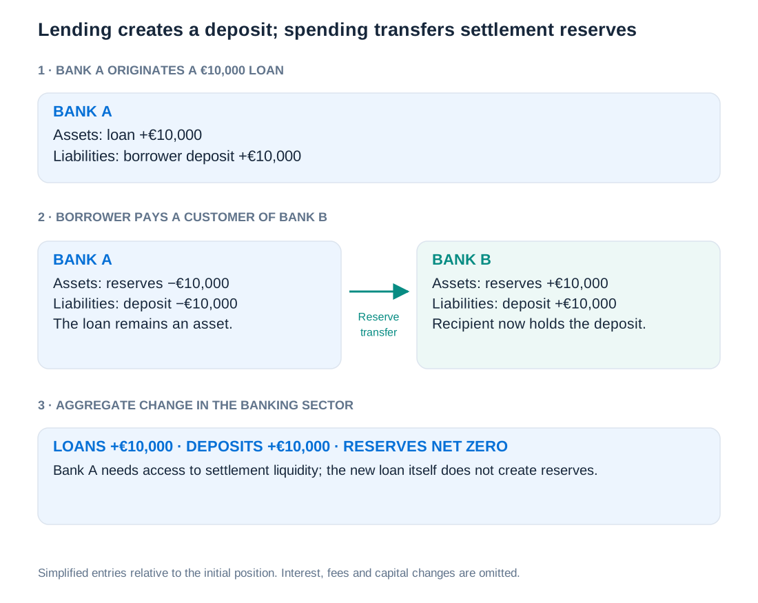
Starting before the loan, the final sector-wide position contains an extra €10,000 loan and an extra €10,000 deposit, with no net increase in reserves caused by the customer transfer itself. This combines the creation and payment exercises into one coherent sequence. If both customers use the same bank, its internal records can transfer the deposit without an interbank reserve transfer. Nevertheless, the bank still has to prepare for later withdrawals and outgoing payments.
The need for settlement funding explains why an individual bank actively attracts deposits. It can also obtain funding through interbank borrowing, securities issuance, secured market borrowing or eligible central-bank facilities. It does not literally require one specific kind of new deposit before every loan can be booked. The accurate conclusion is that lending creates deposits at the system level while the originating bank must manage the funding and liquidity consequences of payments leaving it.
Why bank money cannot expand without limit
A profitable loan must cover funding costs, expected credit losses, operating expenses and the cost of capital and liquidity. Expanding loan demand may require lower lending rates, while attracting stable funding may require higher deposit rates. The resulting compression of margins limits expansion. Poor credit quality can make an apparently high contractual rate unprofitable once defaults and recoveries are considered. A bank also needs enough loss-absorbing capital and eligible liquid assets to satisfy its risk management and regulatory constraints.
These limits operate differently for one bank and for the sector. If only Bank A expands, much of the newly created deposit may leave for competitors. If many banks expand simultaneously, some outgoing deposits are offset by incoming payments. That does not eliminate credit risk, system-wide leverage or the possibility that banks collectively underestimate risk. Capital and macroprudential constraints remain relevant even when the distribution of deposits appears comfortable.
Borrowers and deposit holders provide a second constraint. Creditworthy customers may not want additional debt at the terms offered. Recipients of new deposits may use them to repay existing bank loans, reversing money creation. Third, monetary policy influences the interest rates and financial conditions on which borrowing, saving and portfolio decisions depend. Central-bank support for settlement does not give a commercial bank an unconditional right to borrow unlimited amounts without collateral, eligibility requirements or a viable balance sheet.
Money destruction, asset purchases and the behaviour of deposit holders
Repayment of loan principal using a deposit contracts the banking system's balance sheet: the bank's loan asset and its deposit liability both fall. If the merchant in the €10,000 example uses €4,000 of the proceeds to repay an existing bank loan, the original €10,000 increase in sector deposits is reduced to €6,000, other things equal. A loan loss is different. Writing off an uncollectible loan reduces a bank asset and equity or an existing allowance; it does not automatically cancel the deposit that the original borrower previously spent.
A bank can also create deposits by purchasing a security from a non-bank customer and crediting the customer's account. The new asset is then a security rather than a loan. Conversely, a bank selling a security to a non-bank customer against a deposit can reduce deposit money. When a non-bank investor subscribes to newly issued bank equity or a long-term bank bond using deposits, the bank changes its liability structure: money-like deposits are replaced by equity or debt outside the relevant aggregate. This can improve funding resilience even as measured deposits fall.
If a household merely decides to save rather than spend an existing deposit, the aggregate stock does not necessarily increase. The household retains money that otherwise would have become a firm's deposit. When a recipient repays debt, economists sometimes describe the reversal of deposit creation as reflux. When recipients instead pass unwanted balances to others by buying goods or assets, the process is sometimes called the hot-potato effect. An individual can reduce their deposit by spending it, but the banking-sector deposit normally passes to someone else unless a money-destroying transaction occurs. Prices, spending, desired liquidity and debt repayment jointly determine the eventual adjustment.
Reserves, policy rates and the limits of the money multiplier
Reserves are central-bank liabilities held by eligible institutions, not ordinary household current accounts. A bank can transfer reserves to another eligible participant; it does not lend the same reserve account balance directly to a household. Lending to a household normally creates a bank deposit. Reserve demand follows from settlement needs, regulation, precautionary liquidity management and the opportunity cost of holding balances.
In a deliberately simplified fractional-reserve model, a fixed reserve requirement and a fixed supply of reserves imply a maximum deposit quantity . This requires restrictive assumptions: banks lend up to the limit, the public does not withdraw currency, no excess reserves are held, and reserve supply is the binding exogenous constraint. A broader accounting ratio can be written
where is the model's money stock, its monetary base, the currency-to-deposit ratio and the excess-reserve-to-deposit ratio. Even when this identity is useful, the ratios are not generally fixed behavioural constants.
Modern interest-rate implementation therefore cannot be inferred from a mechanical fixed multiplier. The central bank influences the price of reserve funding, often through remuneration and lending facilities, and supplies or absorbs liquidity under its operating framework. Policy rates feed into money-market rates, deposit and loan prices, asset valuations, exchange rates and expectations. Reserve abundance does not force banks to find creditworthy customers, while expensive funding can restrain credit even when there is no shortage of reserve balances in aggregate. The details differ across monetary systems and over time.
Quantitative easing: a complete balance-sheet example
Quantitative easing (QE) involves central-bank asset purchases, often of government bonds. It became especially important when short-term rates approached their effective lower bound and further conventional easing was constrained. The lower bound is not a universal fixed positive number: holding physical currency has costs, and institutional conditions influence how far rates can fall. The 0.5% UK policy rate discussed in the 2014 account describes that historical setting, not a permanent technical minimum. Consider a stylised purchase of GBP 1 billion of bonds from a pension fund. The fund does not hold an ordinary reserve account at the central bank, so its commercial bank intermediates the settlement. The central bank acquires the bonds and credits the commercial bank's reserve balance; the commercial bank credits the fund's deposit. The entries below omit any separate asset-purchase vehicle and show the consolidated monetary mechanism.
| Entity | Asset changes | Liability changes | Immediate net-worth change at the transaction price |
|---|---|---|---|
| Central bank | Government bonds +1 | Bank reserve balance +1 | 0 |
| Commercial bank | Reserves +1 | Pension-fund deposit +1 | 0 |
| Pension fund | Government bonds −1; deposit +1 | 0 | 0 |
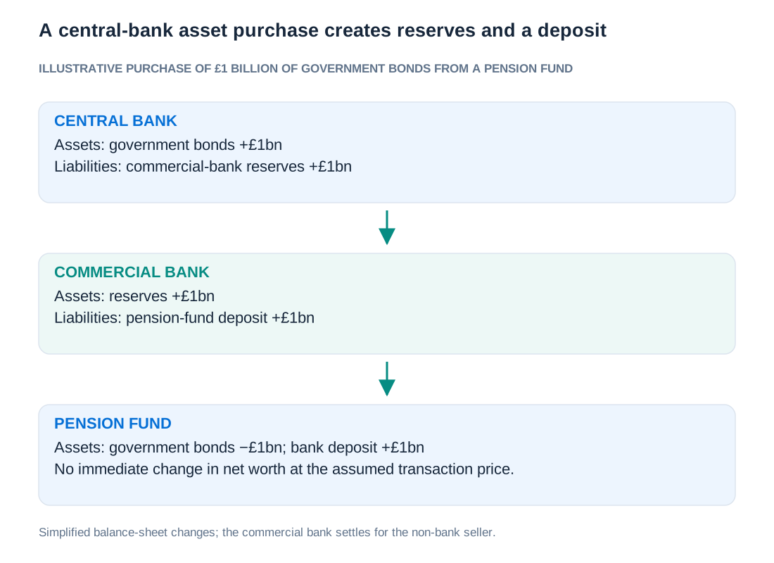
Both reserve money and deposits increase in this example, without a new commercial-bank loan. If the central bank instead buys a bond already owned by a commercial bank, that bank exchanges a bond for reserves; an additional non-bank deposit is not required by that transaction. The identity of the seller is therefore essential.
The pension fund may rebalance away from its larger cash position by buying corporate bonds or equities. Such purchases can affect prices, yields and financing conditions, influencing spending and investment. QE can also operate through expectations and other channels; no fixed ratio converts a given reserve increase into new loans or inflation. It may indirectly encourage bank lending, but a company that raises market finance and repays a bank loan can reduce bank credit instead. The new reserves are not a free addition to bank equity: in the non-bank purchase example they are matched by a deposit liability, and the associated interest income, deposit cost and regulatory effects must all be considered.
Why monetary measurement varies across countries and periods
The Bank of England's 2014 analysis distinguishes several historical UK measures. M0 combined notes and coins with banks' operational balances at the central bank before its publication was discontinued after the 2006 operating-framework reform. Measures such as non-interest-bearing M1, money of zero maturity (MZM), retail M4, M4 and M4ex used different instruments and sectors. M4ex excludes intermediate other financial corporations to reduce the influence of financial-sector intermediation that may be less closely connected to final spending. These are historical statistical definitions, not interchangeable names for euro-area M1, M2 and M3.
| Measure | Main included instruments | Measurement purpose or limitation |
|---|---|---|
| Notes and coin | Currency outside the Bank of England | Narrow indicator of cash-based transactions. |
| M0 | Notes, coin and central-bank reserves | Historical base-money measure; publication changed after the 2006 operating reform. |
| Non-interest-bearing M1 | Currency and non-interest-bearing sight deposits of the non-bank private sector | Can shift strongly when the opportunity cost of non-remunerated balances changes. |
| MZM | Currency and all sight deposits of the non-bank private sector | Zero-maturity balances available without waiting for a term deposit to mature. |
| M2 or retail M4 | Currency and retail deposits, including retail time deposits | Broader household-oriented liquidity measure, with some corporate retail deposits. |
| Historical M3 | Currency and sight and time deposits at banks, excluding building societies | Historical broad-money series; not the euro-area M3 definition. |
| M4 | Currency, deposits, certificates of deposit, repos and eligible securities with maturity below five years held by the non-bank private sector | Broad range of money-like bank liabilities. |
| M4ex | M4 excluding deposits of intermediate other financial corporations | Reduces the weight of intermediation within the financial system. |
| Divisia | Weighted growth of different monetary instruments | Attempts to reflect transaction services rather than giving every instrument the same weight. |
Definitions and publication practices evolve; the table describes the comparison made in 2014, not an assurance that every historical series is still published unchanged. Narrow transaction balances can corroborate current spending, while broader or sector-specific deposits can reveal portfolio adjustment and sometimes provide information about future expenditure. For example, corporate deposit movements may help interpret investment capacity. Repos can resemble secured deposits economically, while collateral used in financing raises further questions about the boundary between money and other liquid assets.
A simple-sum aggregate assigns one pound of weight to one pound in each included instrument. A Divisia monetary index instead weights growth in components according to the monetary services they provide, using opportunity-cost information. A highly liquid, low-yielding transaction balance may provide more transaction services than a higher-yielding less liquid claim. These approaches can diverge during financial innovation or large shifts in interest incentives.
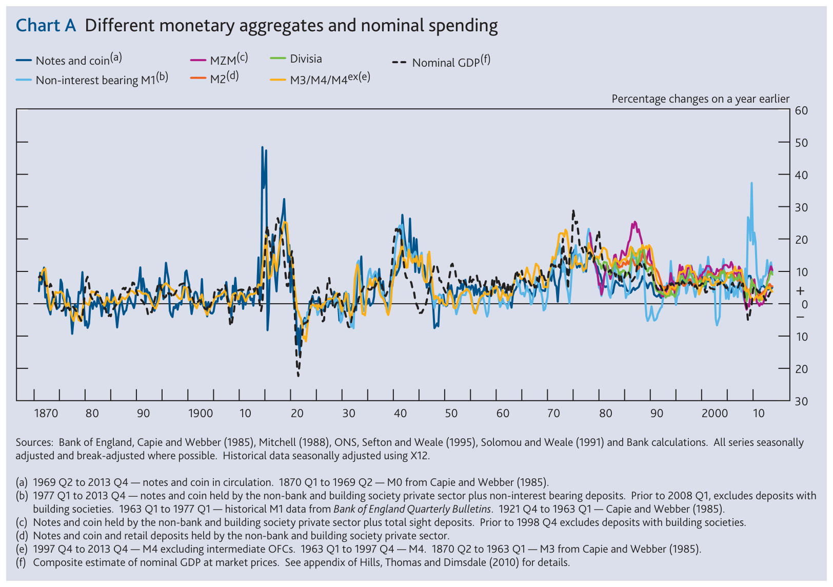
The historical UK comparison shows that monetary aggregates and nominal spending can move together over long periods while diverging sharply over particular episodes. Changes in bank regulation, financial innovation, portfolio preferences, statistical definitions and financial-sector transactions alter the information contained in each series. The accounting relation , with money, velocity, the price level and real output, defines a useful relationship once its components are measured consistently. It does not establish that velocity and output are fixed, or that a money increase translates one-for-one into immediate inflation.
Monetary accounting, constraints, QE and the historical UK comparison are developed from McLeay, Radia and Thomas, Bank of England, Money creation in the modern economy (2014). Its discussion of operating procedures is read in its historical UK setting.
Payment instructions, clearing and final settlement
A payment has several layers. The customer initiates and authenticates an instruction; providers transmit information; clearing determines obligations; settlement discharges those obligations using an agreed asset. A message confirming that an instruction was received is not necessarily final settlement. Finality concerns the point beyond which a transfer is unconditional and irrevocable under the applicable system rules and law. An economic comparison must also consider how mistakes, fraud and customer disputes are handled.
The Single Euro Payments Area (SEPA) harmonises important euro payment instruments across participating jurisdictions. The European Payments Council's credit-transfer and direct-debit schemes specify rules and standards; they are not themselves one universal settlement account. The SEPA Instant Credit Transfer scheme, introduced in 2017, supports transfers available around the clock, with a ten-second execution requirement under the applicable framework. A bank or payment institution connects the customer-facing service to the necessary clearing and settlement arrangements.
T2 is the Eurosystem's real-time gross settlement service, which replaced TARGET2 in March 2023. Gross settlement processes payment obligations individually in central-bank money. The TARGET2 historical annual report for 2022 recorded approximately 108 million transactions with a value of EUR 464 trillion, 99.73% processed in under two minutes and annual costs of EUR 42.7 million. These statistics describe that infrastructure and reporting year; they are neither today's figures nor a retail bank's all-in cost per customer payment.
TARGET Instant Payment Settlement (TIPS), launched in 2018, provides continuous instant settlement in central-bank money. Its published transaction fee of €0.002 is shared between the sending and receiving participants, €0.001 each, under the stated tariff; monthly account-holder fees also apply. That is a settlement-service price, not the entire cost of an account, compliance, fraud prevention, customer support or merchant integration. Participation and account conditions depend on the current framework; one should not assume that every customer-facing provider necessarily has the same access arrangement. Likewise, a scheme participation fee is a membership charge rather than a per-transfer consumer tariff and changes with the relevant fee schedule.
Instant payments: obligations, pricing and customer protection
Regulation (EU) 2024/886 entered into force on 8 April 2024. For the main euro-area credit-institution timetable, receiving instant euro credit transfers was required by 9 January 2025 and sending them by 9 October 2025. Charges for instant transfers may not exceed those for corresponding non-instant transfers, and verification of the intended payee is an important safeguard. Separate timetables and exceptions apply, including for payment and electronic-money institutions and providers outside the euro area. These are phased legal obligations, not a claim that every provider worldwide already offers the same service.
Instant execution reduces waiting time but does not remove fraud. A payer deceived into authorising a transfer may send money extremely quickly to the wrong recipient. Verification of payee, authentication, transaction monitoring, clear warnings and operational resilience complement settlement speed. A credit card or an online wallet can also bundle dispute handling, buyer protection or credit; an account-to-account transfer should be compared with the same service bundle before asserting that one method is universally superior.
Cross-border payments can involve currency conversion, correspondent accounts, compliance checks and institutions operating under different legal regimes. SWIFT mainly provides financial messaging rather than being the money or settlement asset itself. It is also incorrect to treat crypto-assets as intrinsically an infrastructure for illegal activity: they have lawful and unlawful uses, and service providers can be subject to financial-crime controls. The analytical question is which parties perform identification, screening, monitoring and enforcement, and where gaps remain.
Infrastructure and legal references: ECB, T2; ECB, TIPS; TARGET Annual Report 2022; and Regulation (EU) 2024/886. Payment-rule information was checked on 14 October 2026.
10. Stablecoins and Digital Money
A stablecoin is a privately arranged digital token designed to maintain a relatively stable value against a reference, often one US dollar or one euro. The word “stable” describes an objective, not an assurance that the market price can never fall. Understanding a stablecoin requires examining its issuer, reserve assets, redemption rights, ledger, custodians and access points. Its economic role cannot be inferred from transfer speed alone: a fast token can still carry issuer risk, liquidity risk or foreign-exchange risk for the person using it.
Distinguishing monetary claims from their digital representation
Digital money already existed before public blockchains. A bank deposit is usually maintained electronically, while electronic-money institutions issue payment claims under a different legal framework. Tokenisation changes how a claim is recorded and transferred; it does not automatically change the identity of the debtor or the holder's legal rights. A tokenised bank deposit remains a bank liability if that is the legal arrangement. A central-bank digital currency is a public monetary liability. A privately issued stablecoin is a different claim even when all three are denominated in euros.
| Arrangement | Underlying claim | How value is supported | Main analytical question |
|---|---|---|---|
| Commercial-bank deposit | Liability of a commercial bank | Bank assets, capital, supervision and applicable protection arrangements | Can the bank meet withdrawals and absorb losses? |
| Tokenised deposit | Bank deposit represented on a tokenised infrastructure | The legal bank claim and the infrastructure supporting transfer | Do transfer rules preserve the deposit's rights and settlement arrangements? |
| Electronic money | Claim on an issuer received in exchange for funds | Safeguarding, redemption and other applicable legal requirements | Who safeguards the backing and who must redeem the balance? |
| Reserve-backed stablecoin | Private token claim under its issuance arrangement | Reserve value, liquidity and enforceable redemption | Can holders obtain the reference currency at par during stress? |
| Algorithmic stablecoin | Arrangement relying substantially on incentives or linked tokens | Market arbitrage, collateral or issuance rules depending on design | Does stabilisation survive a simultaneous loss of confidence? |
| Retail central-bank digital currency | Direct central-bank monetary liability | Public monetary institutions and its legal framework | How should access, privacy, limits and payment services be designed? |
The relevant comparison is not “digital versus traditional” but the combination of claim, backing, convertibility and transfer architecture. A conventional deposit and a stablecoin can both be accessed through a mobile application, yet expose the user to different institutions. Likewise, a token's address is not necessarily the ultimate beneficial owner: exchanges and custodians may hold balances for many customers.
Reserve-backed, crypto-collateralised and algorithmic designs
A fiat-referenced reserve-backed issuer receives funds and issues tokens against assets such as bank balances, short-term government securities or reverse-repurchase claims. Holders expect conversion into the reference currency under specified conditions. The quality of this promise depends on the assets, segregation and custody arrangements, the legal claim against the issuer and the operational ability to redeem. “Fully backed” is incomplete unless the valuation basis, liabilities included and treatment in insolvency are specified.
A crypto-collateralised design can require collateral worth more than the token liability and liquidate positions when collateral falls. Overcollateralisation provides a buffer, but volatile collateral prices, delayed liquidation, congestion and oracle failures can exhaust it. Algorithmic designs may try to maintain a peg through issuance and redemption against a related token. Such arrangements can become circular: confidence in the stable token depends on the value of the other token, while that token's value depends on confidence in the system. The collapse of TerraUSD in May 2022 is a historical warning that a stabilisation rule can amplify a run rather than absorb it.
Reserve-backed arrangements may resemble narrow intermediaries or money-market funds economically, but the analogy has limits. A fund share can represent a variable claim on net assets; a payment token may promise redemption at a fixed nominal value. Fixed-value redemption makes immediate liquidity and first-mover incentives especially important. A stablecoin also need not offer the deposit insurance or central-bank liquidity access associated with a qualifying bank deposit.
Issuance, transfer and redemption on the issuer's balance sheet
Consider a simplified issuer that receives EUR 1 million and mints one million tokens, each redeemable for one euro. Its assets rise by EUR 1 million and its token liabilities rise by the same amount. No profit arises merely from minting the liability. If one holder transfers 100 tokens to another, the issuer's total assets and total token liabilities are unchanged; only the identity of the holder changes. When 100 tokens are redeemed and cancelled, reserve assets and token liabilities both fall by EUR 100.
| Transaction | Issuer assets | Issuer token liabilities | Effect on issuer equity |
|---|---|---|---|
| Receive EUR 1 million and issue one million tokens | +EUR 1 million cash or eligible reserve assets | +EUR 1 million | No immediate change |
| Transfer 100 tokens between holders | No change | No change in total | No change |
| Redeem and cancel 100 tokens at par | −EUR 100 | −EUR 100 | No change if assets realise par |
| Reserve assets suffer a EUR 20,000 loss | −EUR 20,000 | No automatic reduction | −EUR 20,000 |
The reserve-coverage ratio is
A ratio of 100% on one date is not equivalent to uninterrupted liquidity or an adequate capital buffer. A balance sheet containing EUR 100 million of assets and EUR 100 million of token liabilities has no cushion in this stripped-down example. Custodian fees, operational expenses, asset losses or undisclosed senior claims could undermine the promise unless funded separately.
At the banking-sector level, buying a stablecoin can initially transfer a customer's deposit to the issuer's bank account rather than destroy deposits. If the issuer then buys a security from a non-bank investor, the deposit passes to that seller. Other transactions can change deposits, and the type and concentration of deposit funding can change even when the aggregate does not. It is therefore too simple to say that every euro entering a stablecoin permanently removes one euro from the banking system.
Historical growth and the dominance of dollar denomination
Market capitalisation measures the outstanding token quantity multiplied by its market price. For a token trading close to par, it is a useful approximation to outstanding issuance. It is not annual revenue, transaction value or the issuer's equity value. A stablecoin can be transferred repeatedly during a year, so a relatively small outstanding stock can support a large gross flow. Conversely, large trading activity can reflect exchange transfers, automated operations or movements within an intermediary rather than purchases of final goods and services.
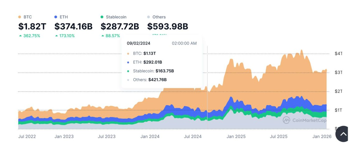
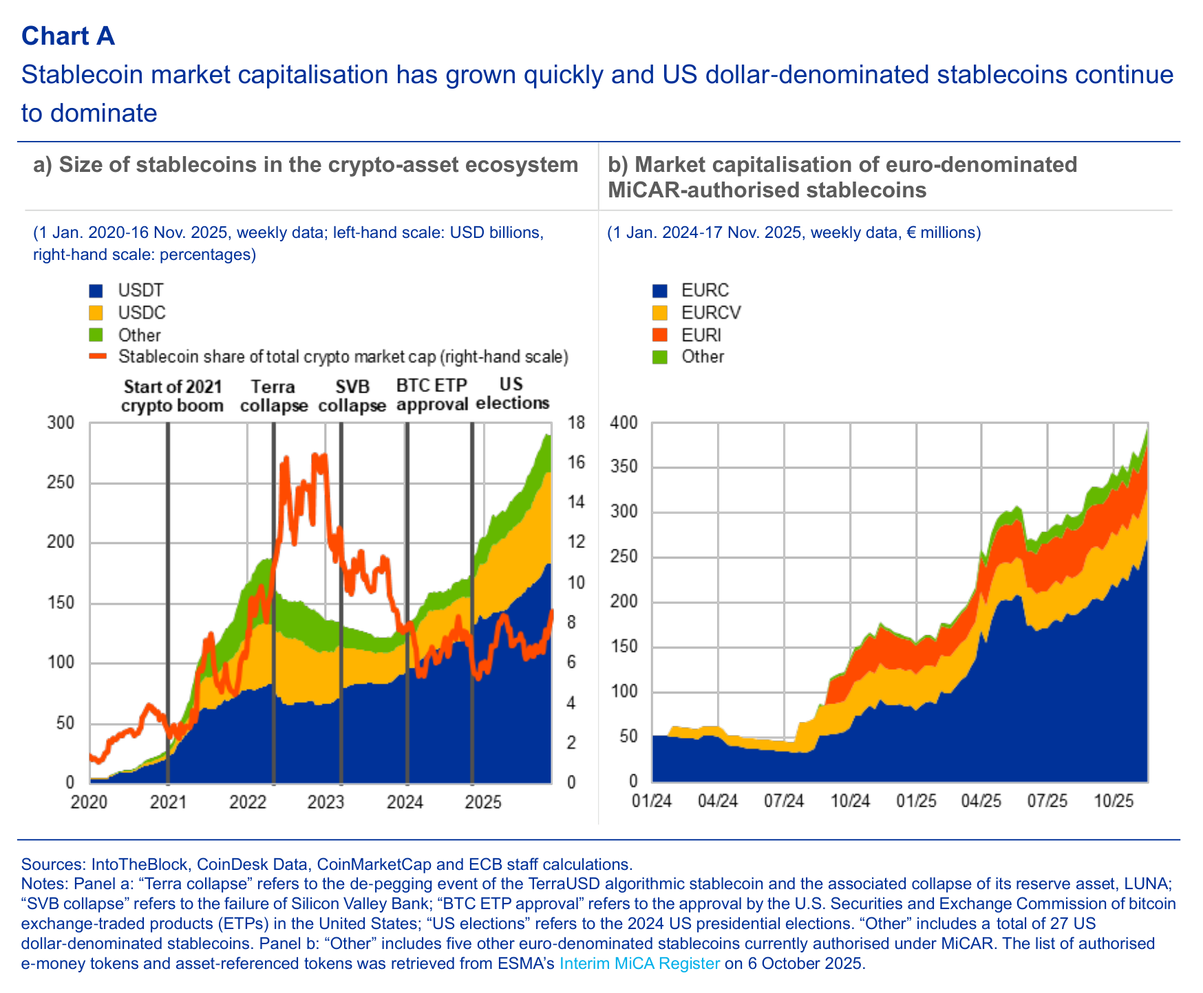
The historical comparisons show the strong role of US-dollar-linked stablecoins and the much smaller scale of euro-linked issuance. This reflects existing dollar use, crypto-market trading conventions, liquidity and issuer networks; the chart alone does not identify the causal contribution of each factor. The euro and dollar panels must be read with their respective units, because millions of euros and billions of dollars are not interchangeable scales.
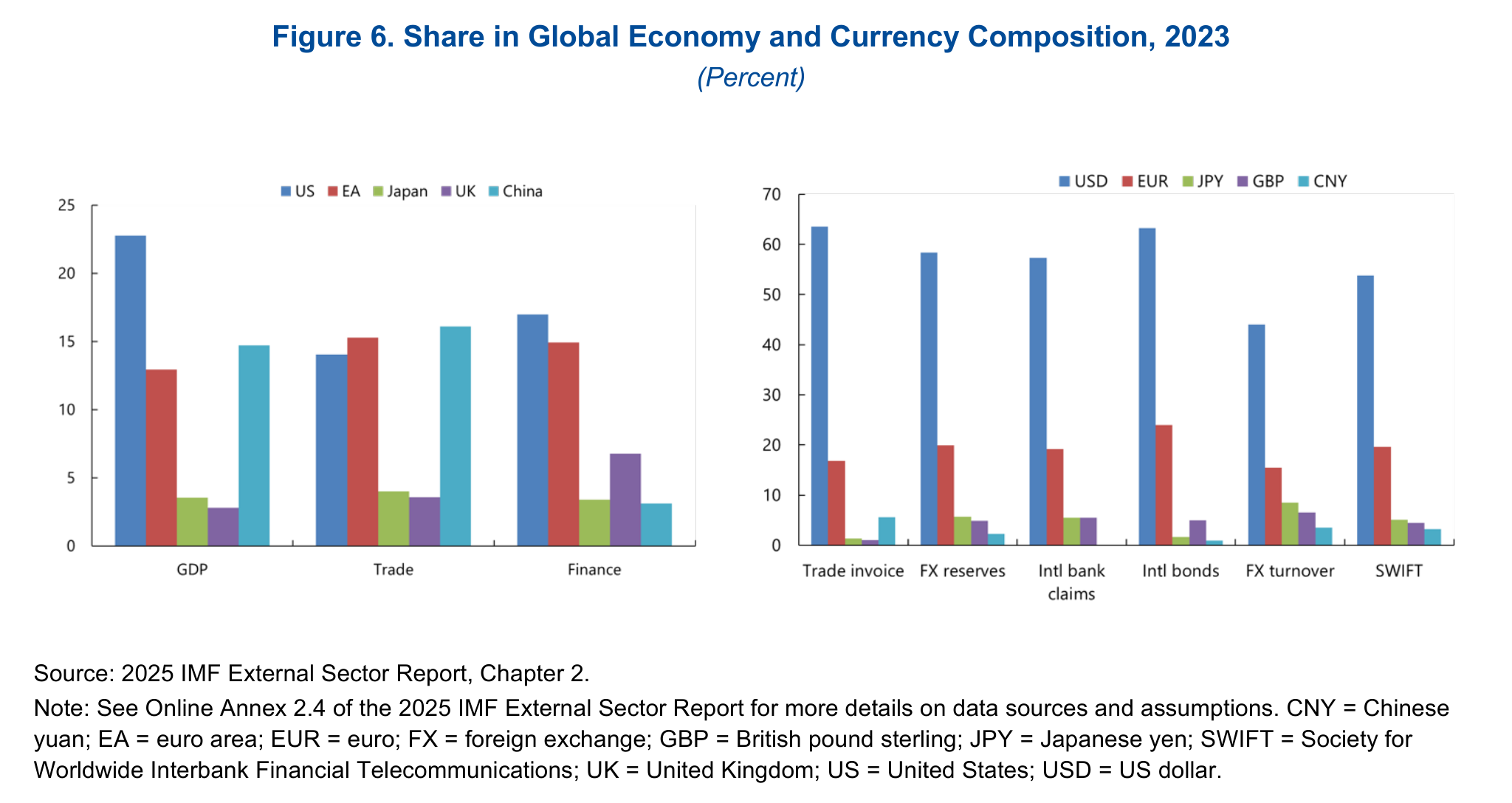
A currency's international role need not match the issuing economy's share of world output. Trade invoicing, foreign-exchange reserves, bank claims, bond issuance, foreign-exchange turnover and payment messages measure different functions, frequently with different denominators. The historical 2023 comparison provides context for stablecoin dollarisation; it is not evidence that stablecoins themselves created the dollar's established international position.
Reserve composition, disclosure and the meaning of assurance
A reserve portfolio composed of short-dated government securities is exposed to different risks from one containing unsecured corporate claims or volatile crypto-assets. Yet even high-quality securities have market prices and settlement times. Maturity, interest-rate sensitivity, currency matching, concentration in particular banks, custody access and encumbrance all affect whether assets can meet redemption requests. A reverse repo is a contractual secured claim, not literally the same balance-sheet item as a Treasury bill held outright.
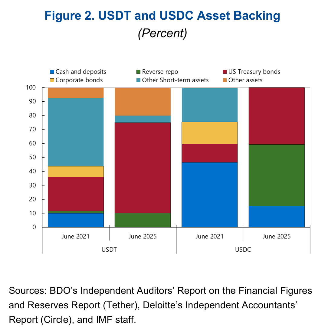
The June 2021 and June 2025 reserve comparison illustrates that backing composition changes over time. Reading a percentage bar requires identifying both the asset categories and what the report covers. An assurance or attestation engagement on a reserve statement at a specified date should not be described automatically as a full audit of every aspect of an issuer's financial statements, internal controls and future liquidity. The report's scope, criteria, date and qualifications determine what can reasonably be concluded.
How a secondary-market peg is maintained and lost
When a token trades below its redemption value, an eligible arbitrageur may buy it and redeem it at par. When it trades above par, an eligible issuer customer may acquire new tokens at par and sell them. These trades tend to narrow deviations, but only if issuance and redemption are accessible, predictable and economical. Minimum transaction sizes, identity checks, banking hours, redemption fees, transfer restrictions or doubts about reserves can interrupt the mechanism. A retail holder selling through an exchange may not have the same direct redemption access as an institutional customer.
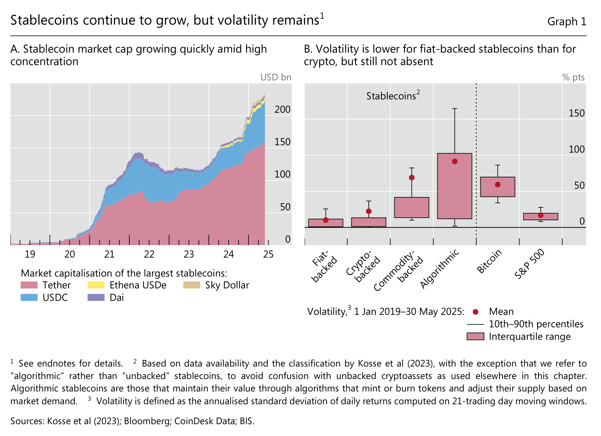
A temporary discount can reflect liquidity constraints rather than a final loss on every reserve asset; a persistent discount can reflect a genuine solvency problem. Distinguishing the two requires evidence. The March 2023 USDC stress illustrates the connection between token confidence and the banks holding reserve cash: uncertainty about access to cash can affect a token trading continuously even while conventional banking operations are constrained. Neither a return to par nor a short historical period of stability proves immunity to future runs.
Worked example: full backing and a redemption shortfall
An illustrative issuer has EUR 100 million of token liabilities, EUR 15 million of immediately available cash and EUR 85 million of securities carried at par. Holders request redemption of 25% of the tokens, or EUR 25 million. The immediate cash shortfall is EUR 10 million. If securities can be sold at par, the issuer sells EUR 10 million, pays EUR 25 million and finishes with EUR 75 million of securities backing EUR 75 million of tokens.
Now suppose an urgent sale produces only 98% of the securities' carrying value, while the unsold securities retain their carrying value for this isolated example. Selling EUR 10 million of face value is insufficient because it raises only EUR 9.8 million. The required sale is
The realised loss is EUR 0.2040816 million. After redemption, remaining assets equal EUR 74.7959184 million while token liabilities equal EUR 75 million. The remaining coverage ratio is approximately 99.728%.
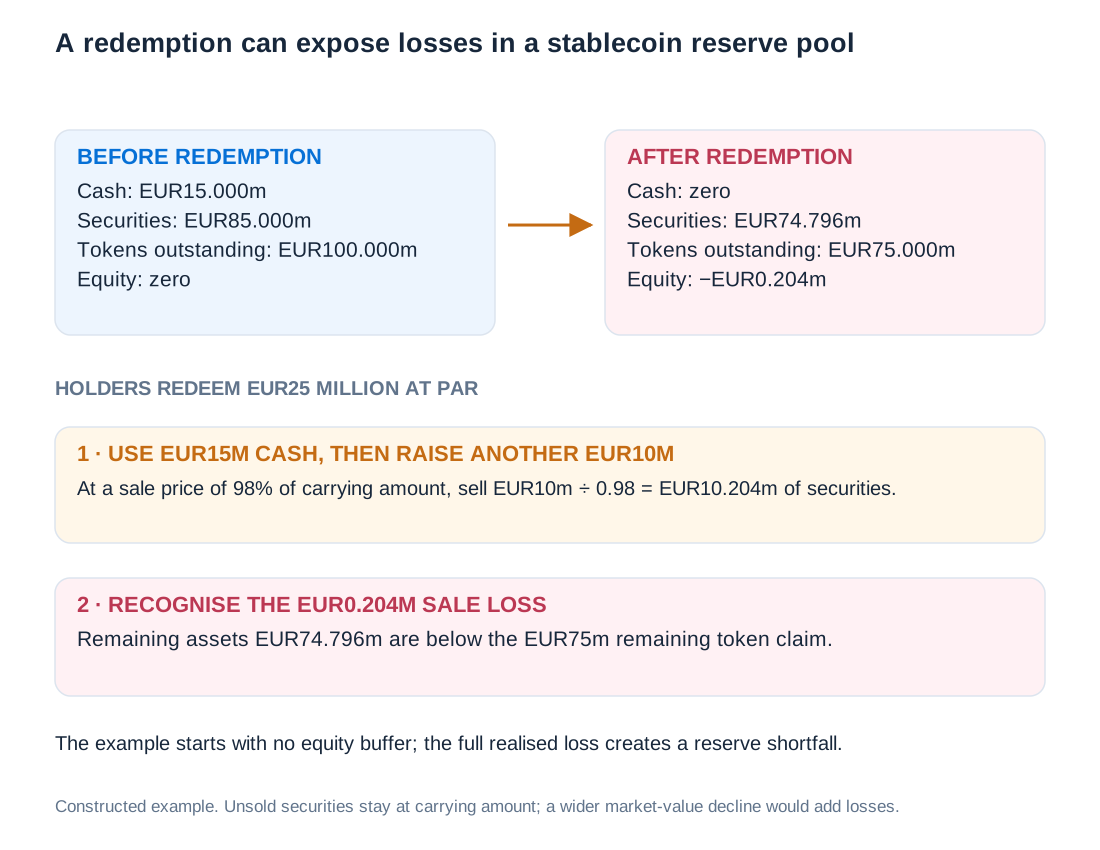
The shortfall is caused by liquidation losses, not by an arithmetic failure to hold EUR 100 million before the run. A separately funded capital buffer of EUR 0.3 million would absorb this particular loss, leaving about EUR 0.0959 million, but would not eliminate other risks. If the price decline also applies to unsold assets, total losses are larger. The example explains why regulation and risk management assess reserve liquidity, valuation, capital and redemption arrangements separately.
Cross-border uses, currency substitution and financial spillovers
Stablecoins can provide a settlement medium within crypto markets and a transferable claim across providers using compatible networks. They may also be useful in particular remittance or business-payment corridors where conventional services are slow, expensive or difficult to access. The complete service still requires conversion, customer identification, secure custody and an accessible endpoint. A token arriving instantly is not equivalent to the recipient having immediately spendable local currency.
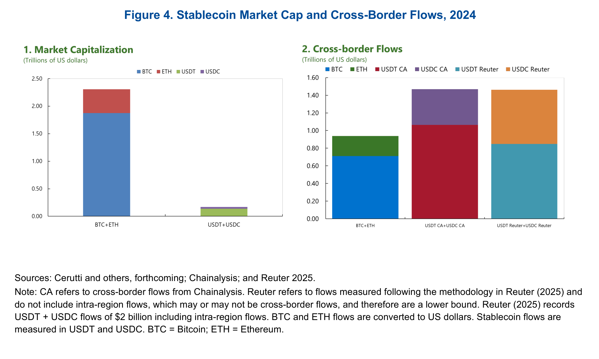
Cross-border estimates depend on identifying where senders and recipients are located, which is difficult when addresses are pseudonymous and exchanges pool customer balances. Gross flows can include repeated transfers and financial trading. The 2024 historical comparison therefore retains alternative estimates and methodological notes instead of presenting one number as a precise measure of global retail remittances.
For a euro-income household, holding a dollar stablecoin adds exchange-rate risk even if the token tracks one dollar perfectly. Widespread foreign-currency token use can support currency substitution, affecting the denomination of prices, savings and contracts. The consequences for domestic monetary policy depend on scale and on what users replace. Access to a foreign unit of account may benefit individuals facing unstable local purchasing power, while creating challenges for the domestic monetary system.
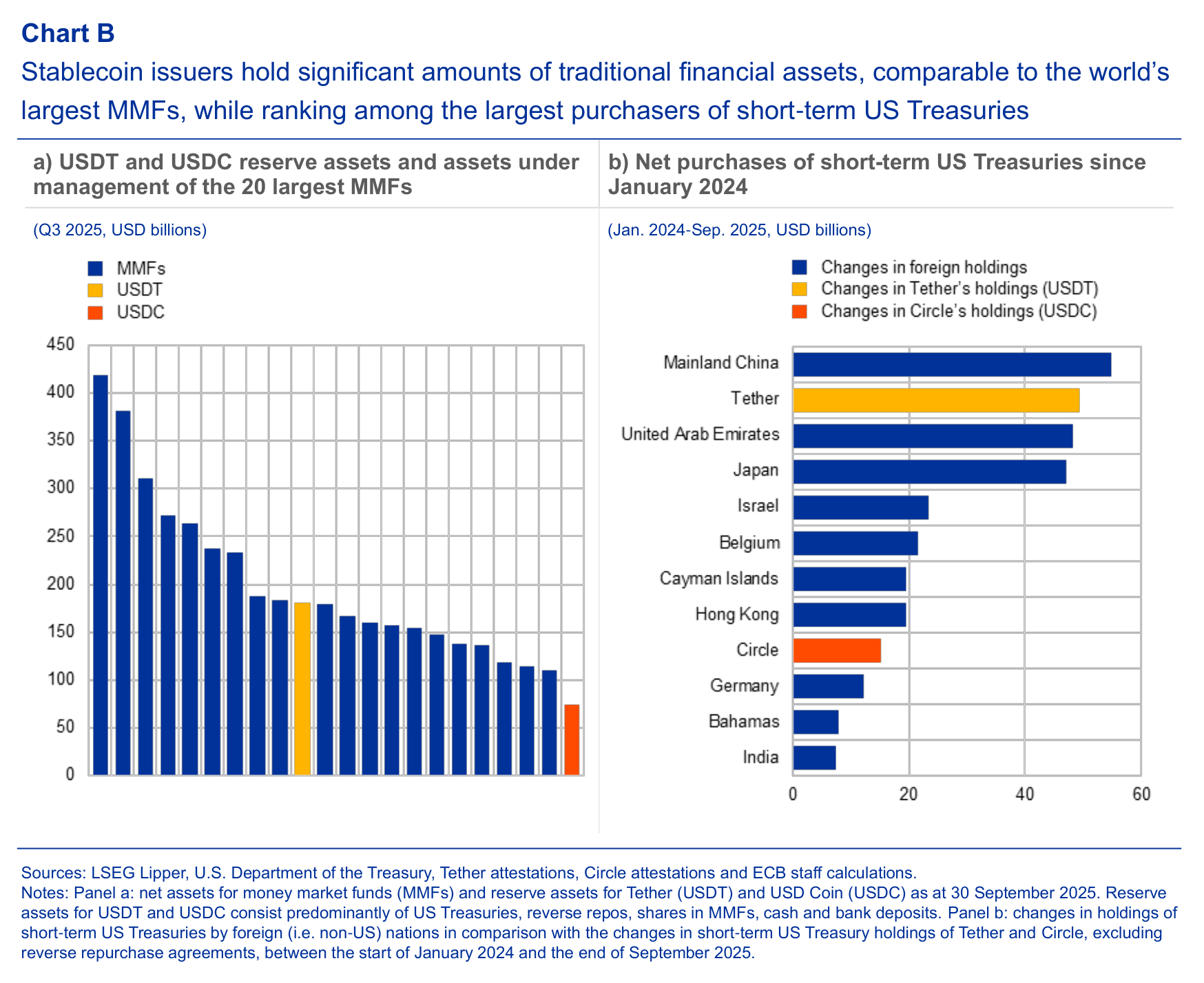
Large reserve portfolios connect stablecoins with banks, money-market funds and government securities. New issuance can increase demand for short-term safe assets; redemptions can require sales or repo unwinding. Empirical estimates of yield responses depend on the sample, shock definition and identification method, and confidence bands must be retained. They do not establish that every inflow lowers yields by a fixed amount, or that every policy-rate increase mechanically causes the same token outflow.
Comparing the full cost of a payment
A fair comparison begins with a specific payer, recipient, currency pair, amount and service requirement. A blockchain fee is one component, while an exchange spread, fiat deposit fee, withdrawal charge, custody service, failed transaction, compliance process or dispute can add others. Conventional providers also differ: a low-cost domestic instant transfer is a different benchmark from a high-friction international retail corridor.
For an illustrative EUR 1,000-equivalent remittance, assume an on-ramp fee of 0.5% (EUR 5), a network fee of EUR 0.50, an off-ramp fee of 0.7% (EUR 7) and an exchange spread of 0.4% (EUR 4), each percentage applied to the original amount for simplicity. Total cost is EUR 16.50, or 1.65%, not merely the EUR 0.50 network fee. A conventional quote of EUR 12 would be cheaper under these assumptions; a quote of EUR 25 would be more expensive. Neither comparison tells us about fraud remedies, execution risk or recipient accessibility unless those features are also specified.
| Dimension | Question to answer | Common misleading shortcut |
|---|---|---|
| Total monetary cost | What does the recipient receive after all fees and exchange spreads? | Comparing only blockchain gas with a bundled bank fee |
| Time | When can the recipient actually use the final currency? | Treating ledger confirmation as completed fiat withdrawal |
| Legal finality | When is the obligation discharged under applicable rules? | Equating a technical confirmation with every legal consequence |
| Consumer protection | Who handles fraud, mistakes and merchant disputes? | Assuming irreversibility is always a consumer benefit |
| Liquidity and credit | Who supplies prefunding, currency conversion and settlement balances? | Assuming intermediaries and liquidity costs disappear |
| Operational resilience | What happens during an outage, key loss or provider failure? | Assuming a decentralised ledger removes all concentrated dependencies |
Atomic settlement, smart contracts and incomplete agreements
Tokenisation can make payment and asset transfers conditional on each other. In delivery-versus-payment, securities should move if and only if the payment leg moves; in payment-versus-payment, the two currency legs are linked. Atomic execution can reduce principal risk arising from one party delivering while the other does not. It does not remove the need for legally enforceable ownership, authorised issuers, custody, access controls and recovery procedures. Requiring both legs to be fully prefunded can also increase liquidity needs compared with arrangements that permit netting or intraday credit.
A smart contract executes a rule using available digital inputs. Paying a freelancer when a file is uploaded is easy to encode; determining whether the work satisfies a disputed quality standard is harder. A supply-chain contract needs reliable evidence that the right goods arrived in acceptable condition. An oracle introduces external information, but then the system depends on that source's accuracy and governance. Automation reallocates some trust; it does not abolish trust.
Conditional payments should also be distinguished from programmable money restricted to particular purposes, dates or recipients. A customer can voluntarily instruct a payment on delivery while holding general-purpose money. Technology can reduce reconciliation and automate well-specified processes, but commercially meaningful agreements remain incomplete and require dispute resolution. A legal remedy can remain necessary even when the ledger transfer itself is technically irreversible.
The European regulatory categories
Under the EU Markets in Crypto-Assets Regulation (MiCA), a token seeking stable value by reference to one official currency falls within the e-money-token category; asset-referenced tokens use a different reference structure. E-money-token issuers must generally be authorised credit institutions or electronic-money institutions. Tokens are issued at par on receipt of funds, holders have a right to redemption at par, and issuers may not grant interest linked to the holding period. The regulation imposes additional requirements on reserves, governance and disclosures according to the relevant category. Its stablecoin provisions applied from 30 June 2024, with most other provisions applying from 30 December 2024.
A legal label does not eliminate operational or market risk. The holder still needs to identify the issuer and understand custody and redemption. A token should not be described as an insured bank deposit simply because a bank is involved. Rules also differ across jurisdictions, so the rights attached to one regulated European arrangement should not be projected onto every token bearing the same currency name.
Legal reference: Regulation (EU) 2023/1114 (MiCA), notably the categories and the e-money-token provisions. Legal description checked on 14 October 2026.
Evaluating claims about financial innovation
An implemented product, a pilot and a proposed use case are different forms of evidence. A persuasive assessment defines the problem, identifies a realistic existing alternative, measures the complete cost and risk allocation, and states circumstances in which the result would reverse. Market capitalisation is evidence of valuation or issuance, not proof of welfare improvement. A demonstration of technical feasibility is not evidence of broad adoption, and a correlation between token flows and financial prices is not automatically causal.
The same discipline applies to automated research and generative-AI output. Fluent explanations can confuse a ledger with a currency, an attestation with an audit, or a fee comparison with a full welfare assessment. Each claim needs a source appropriate to the question: legal texts for rights, audited reports for financial statements, system documentation for operating rules, and research with a credible identification strategy for causal effects. Stablecoins are best understood as institutional arrangements whose benefits and vulnerabilities must be assessed together.
Historical evidence and interpretation: IMF, Understanding Stablecoins (2025); ECB, Stablecoins on the rise (November 2025); and BIS, Annual Economic Report 2025, Chapter III. Graphs retain their historical samples rather than being presented as current market data.
11. Innovation and Competition in Payments
Payments are a financial service, a technology business and a coordination problem. Customers want a convenient and trustworthy way to pay; merchants want completed sales at an acceptable cost; providers need enough revenue to finance infrastructure, fraud control and support. The same transaction can involve a wallet, a card scheme, an acquiring bank, an issuing bank and central-bank settlement. Innovation can improve one layer without replacing the others, which is why a familiar bank account can remain behind a new customer-facing application.
The layers of a payment service
The interface determines how a person initiates a payment, whether with a card, application, QR code or online checkout. Authentication establishes who is authorising it. Messaging communicates the instruction; clearing calculates obligations; settlement discharges them using an agreed asset. Merchant acceptance, compliance, dispute handling and customer service connect these layers to real commercial activity. A provider may specialise in one function or integrate several.
Consider a mobile wallet that tokenises a customer's existing card credentials. The consumer may experience a new and convenient product, while the payment continues to use a card network and a bank account. Consequently, wallet use and card use can overlap. They must not be added as if they were mutually exclusive payment categories. An account-to-account service can instead initiate a credit transfer, but still needs authentication, fraud controls and merchant reconciliation.
| Layer | Economic role | Example of a relevant performance measure |
|---|---|---|
| Customer interface | Make payment initiation convenient and accessible | Checkout completion, time and accessibility |
| Authentication and risk control | Limit unauthorised use and fraud | Fraud losses, false declines and recovery |
| Acceptance and scheme rules | Connect payers and merchants under shared rules | Active acceptance, coverage and interoperability |
| Clearing and settlement | Determine and discharge financial obligations | Finality, liquidity use, uptime and settlement failures |
| Post-payment services | Resolve disputes and reconcile transactions | Resolution time, refund handling and support cost |
| Credit and value-added services | Provide financing, loyalty or other complementary services | Incremental benefit after credit losses and service costs |
Two-sided markets and cross-side network effects
A payment platform usually serves at least two interdependent groups. Consumers value a method more when many merchants accept it; merchants value it more when many customers actively use it. These are cross-side, or indirect, network effects. Direct network effects instead arise when users benefit from other members of the same group, as with person-to-person messaging or transfers. Both can exist in a payment ecosystem, but they are analytically distinct.
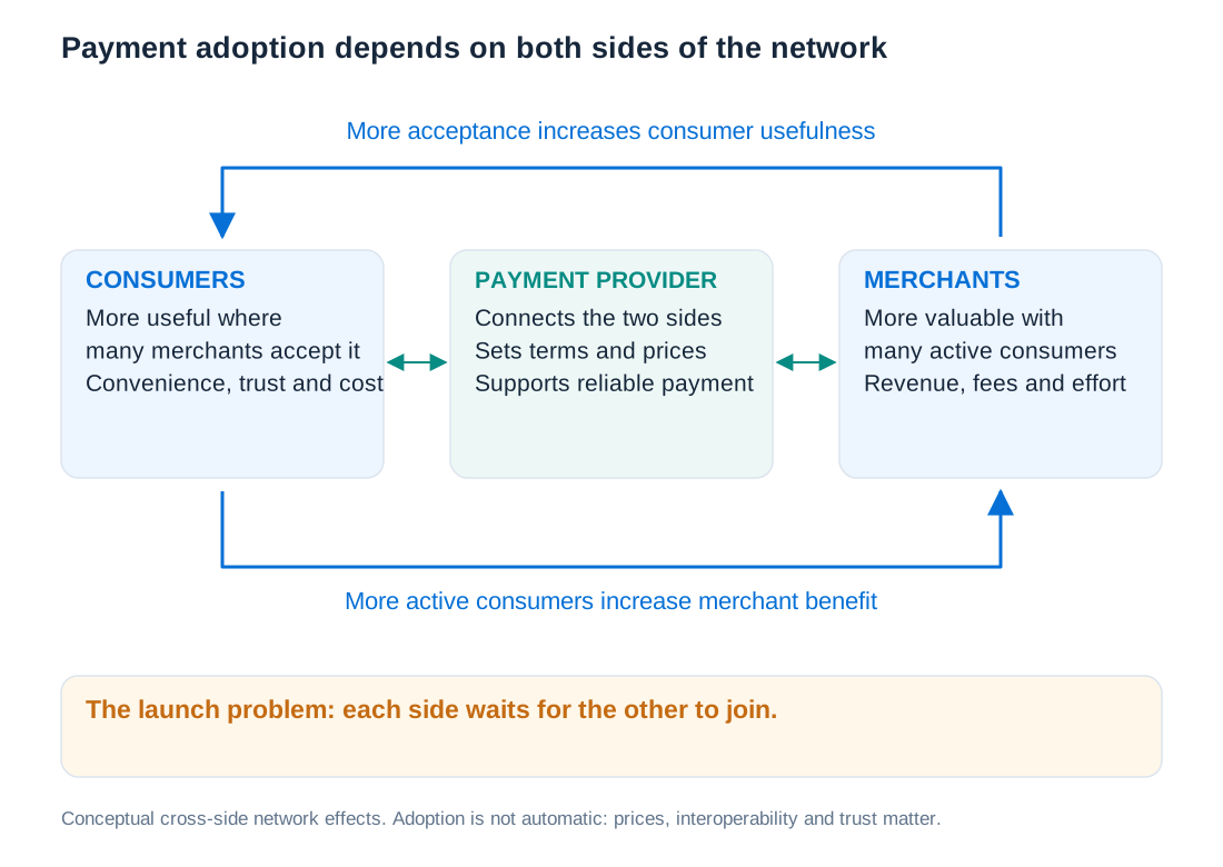
A technically excellent method with few accepting merchants gives consumers little reason to adopt. Merchants, in turn, may refuse integration until consumer demand exists. This coordination problem explains why a new platform may subsidise one side, recruit anchor merchants or integrate into an application with an existing user base. It also explains why charging each side its narrowly measured processing cost need not maximise adoption or profit.
A simple representation is , where consumer utility rises with the number of relevant merchants , falls with the consumer price , and falls with adoption frictions . Merchant benefit can similarly be written . The parameters and capture cross-side benefits in a stylised model, not estimated universal constants. The relevant counts are usable, active counterparties rather than every registered account worldwide. A high nominal user count can be commercially unhelpful if those users never select the method.
Positive feedback can make established networks difficult to displace, but concentration is not inevitable. Consumers and merchants can multi-home, using several providers, and interoperability can connect networks. Switching costs, exclusive arrangements, default settings, device access and the cost of integrating additional methods affect competitive pressure. Network effects and economies of scale are also different: network effects change the value of participation, whereas economies of scale reduce average cost as output increases.
Solving a customer problem before pursuing scale
Successful innovation removes a specific friction. Early e-commerce created problems of trust, repeated data entry, unfamiliar merchants and abandoned checkout. A wallet that simplifies payment and provides credible dispute handling can create value without inventing a new settlement asset. A merchant may accept a higher fee if the service brings additional profitable sales, reduces fraud or improves reconciliation. The gain must be measured against an appropriate alternative, not against a world in which payment has no cost.
Operational details are central to this value proposition. A mobile-first design can lower entry friction, while accessible authentication can improve inclusion. Poor refund handling, outages or wrongful account restrictions can destroy the benefit of rapid execution. For a credit-linked product such as buy now, pay later, convenience and conversion must be assessed together with underwriting, expected losses, consumer indebtedness and funding costs. A payment feature and a credit feature are complementary services, not the same product.
The useful metrics therefore include active users, transaction frequency, merchant acceptance, conversion, fraud-adjusted contribution, retention and acquisition cost. Download counts and registered accounts provide incomplete information. A controlled rollout or credible comparison group is more informative about incremental sales than observing that highly engaged customers spend more: customers may join a loyalty programme precisely because they already buy frequently.
Payment mixes in 2024: value, volume and channel
Offline and online retail have different transaction needs. Physical cash can be useful at a point of sale but cannot be handed directly to a remote merchant. Online wallets, invoices and account transfers can therefore occupy a larger role in e-commerce, while card form factors differ between physical and digital checkout. Moving a sale online can change which provider controls the customer relationship even if bank money still funds the final transaction.
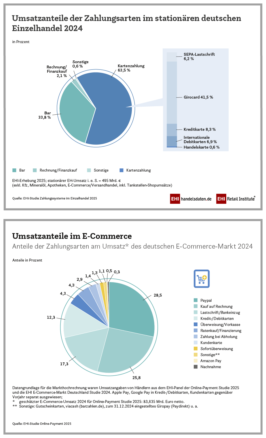
The two 2024 snapshots compare payment methods within each channel; they are not a time series. The physical-retail chart separates cash, card-based payments, invoice or financing purchases and other methods, and then breaks down the card-based category. The e-commerce chart distinguishes PayPal, invoice payment, direct debit, credit and debit cards, advance transfers, instalment financing, payment on collection, customer cards, immediate-transfer services, other methods, Amazon Pay and cash on delivery. Shares use the respective channel’s transaction value; the populations and reporting basis are not identical.
| Channel | Method | Share | Interpretation |
|---|---|---|---|
| Physical retail | Cash | 33.8% | Value share differs from the 54.6% share of transaction count. |
| Physical retail | Girocard | 41.5% | Domestic card category. |
| Physical retail | International debit cards | 6.9% | Separate from Girocard in this classification. |
| Physical retail | Credit cards | 8.3% | Separate from debit cards. |
| Physical retail | SEPA direct debit | 6.2% | The published classification distinguishes it from the other card categories. |
| Physical retail | Other methods | 3.3% | Residual after the displayed rounded shares. |
| E-commerce | PayPal | 28.5% | Value share in the online comparison. |
| E-commerce | Invoice payment | 25.8% | Payment after invoicing. |
| E-commerce | Direct debit | 17.3% | Account-based collection. |
| E-commerce | Credit and international debit cards | 12.3% | The online grouping differs from the offline grouping. |
| E-commerce | Other methods | 16.1% | Includes the remaining online methods. |
The cash result illustrates the importance of denominators: cash can account for most purchases by number while representing a smaller share of their combined value because cash transactions tend to be smaller. The table also corrects a common classification mistake: the online card category includes international debit cards, so it should not be labelled simply “credit cards”. These are historical survey results for 2024, not current shares or a complete census of every payment. In the full graphics, the physical-retail value basis is EUR 495 billion, while the e-commerce estimate is EUR 83.835 billion net of tax. Their percentages can be compared within their respective definitions, but their euro totals should not be added without harmonising scope and tax treatment.
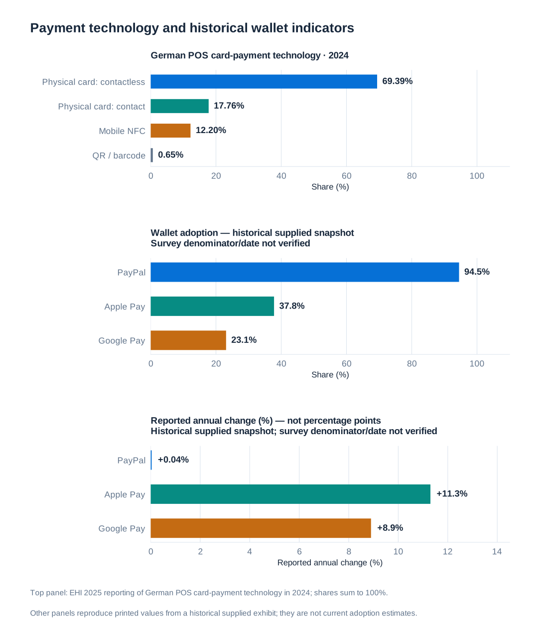
Form-factor penetration provides another perspective. Contactless physical cards, chip-based cards and mobile wallets describe how customers initiate payments. Merchant availability of a wallet, consumer adoption of a wallet and its share of actual purchases are different quantities. Multiple-wallet adoption rates can sum to more than 100%, while mutually exclusive transaction shares should sum to approximately 100% after rounding. Historical wallet charts must therefore retain their survey population and definition; where these are not specified, they illustrate categories rather than support a precise population-wide estimate.
Historical retail data: EHI Retail Institute, Zahlungssysteme im Einzelhandel 2025 and Online-Payment 2025, both reporting 2024 activity. The final category in each group is the residual of the displayed rounded shares.
Revenue, payment volume and profit are different quantities
Payment value is the amount transferred for customers, not the provider's revenue. If a provider handles EUR 1 billion and earns EUR 10 million, its revenue take rate is 1%. If it earns EUR 2 million of profit, profit is 0.2% of payment value but 20% of revenue. The denominators answer different questions. Confusing them can produce comparisons that exaggerate or conceal differences in business models.
Illustrative historical comparison figures of 0.2% or 0.3% for a card-related charge, 1.74% for wallet revenue and 2.7% for a credit-linked service are not interchangeable measures. Interchange is only one component of a merchant's total payment cost, while a wallet or credit product can combine processing, buyer protection, financing and other services. Likewise, illustrative profit-to-payment-value ratios of 0.05%, 0.52% and 1.5% do not establish directly comparable corporate profit margins. Without matched dates, geography, product scope and accounting definitions, such figures should be used to explain measurement, not rank named providers.
For example, if a provider has revenue equal to 1.74% of payment value and profit equal to 0.52% of the same payment value, the implied profit margin on revenue is
This is valid arithmetic under the stated assumptions, not a verified current margin of a particular company. Consolidated profit can also contain activities unrelated to payment processing, while transaction margins may exclude acquisition and fixed infrastructure costs.
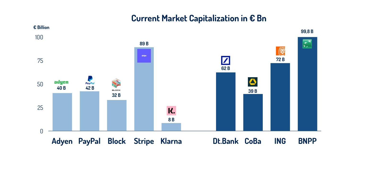
The historical valuation comparison shows that payments can support large standalone businesses, but equity valuation is a stock reflecting expected future cash flows and risk. It is not payment throughput, a bank's asset size or regulatory capital. Private funding-round valuations may be infrequent and attach to securities with different rights; they are not necessarily comparable with the continuously traded market capitalisation of common shares. A valuation chart therefore raises questions about business models rather than proving that one business is economically superior.
Worked example: contribution, fixed costs and break-even volume
Suppose a provider processes 50 million transactions annually, earning average revenue of EUR 0.18 and incurring variable cost of EUR 0.11 per transaction. The contribution per transaction is EUR 0.07. Total revenue is EUR 9 million, variable cost is EUR 5.5 million, and contribution before fixed expenses is EUR 3.5 million. This is the integrated payment-pricing example; calling the EUR 3.5 million “net profit” would omit necessary costs.
Let be the number of transactions, revenue per transaction, variable cost per transaction and annual fixed expenses. Then
With , annual operating profit is EUR −0.5 million. If the per-transaction assumptions remain unchanged, break-even volume is
Processing another 10 million transactions adds EUR 0.7 million of contribution, turning profit into EUR 0.2 million if it requires no additional fixed capacity.
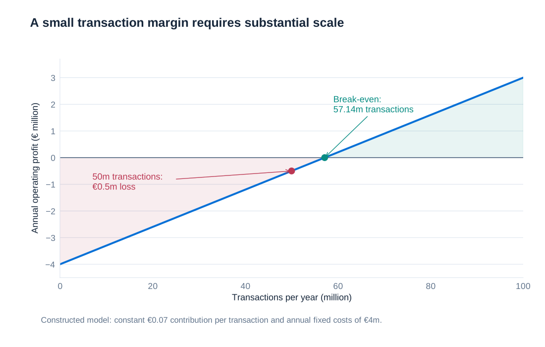
The constant-cost assumption is only a starting point. Fraud losses may rise, higher-risk merchants may join, compliance costs may increase, or price discounts may be needed to attract volume. If the variable cost rises to EUR 0.14, the margin becomes EUR 0.04 and break-even volume increases to 100 million transactions. If , more volume cannot cover positive fixed costs under the unchanged model. Growth creates value only when its incremental benefits exceed its incremental costs.
Loyalty payments: the Starbucks case
A merchant wallet can combine payment, loyalty rewards and ordering. Prepayment supplies funds before goods are delivered; mobile ordering can reduce checkout friction; rewards may encourage repeat use. These mechanisms are economically distinct. A customer's unspent balance is initially an obligation to provide future goods or services, not immediate sales revenue. Nor does receiving prepaid customer balances by itself turn a retailer into a deposit-taking bank.
Starbucks' fiscal 2024 reporting records loaded card amounts as deferred revenue until redemption and recognises estimated unredeemed balances, or breakage, according to its accounting policy and applicable unclaimed-property requirements. Its combined stored-value and loyalty liability reconciles as follows.
| Item | Amount | Interpretation |
|---|---|---|
| Opening balance, 1 October 2023 | 1,567.5 | Existing deferred obligations |
| Activations, reloads and Stars earned | +15,807.1 | Newly deferred revenue |
| Card and Stars redemptions and breakage | −15,665.1 | Revenue recognised and obligations reduced |
| Other movements | +9.2 | Primarily currency translation |
| Closing balance, 29 September 2024 | 1,718.7 | Remaining combined obligation |
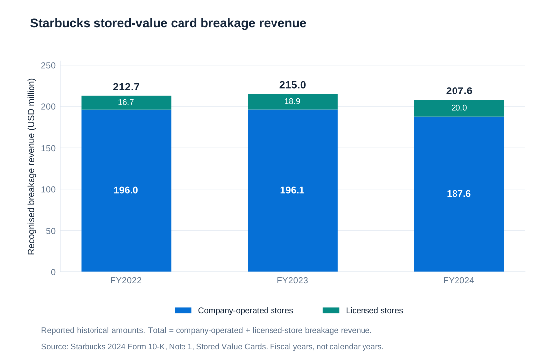
The breakage series totals USD 212.7 million in fiscal 2022, USD 215.0 million in 2023 and USD 207.6 million in 2024. It does not rise in every year. These totals combine company-operated and licensed-store revenue and are distinct from interest earned on invested cash. The combined liability table also includes loyalty Stars, so it should not be described as a pure balance of unused gift-card cash.
A retailer may benefit economically from the interval between receiving cash and supplying goods: holding cash can generate investment income or reduce financing needs. That benefit depends on rates, cash management and costs; it should not be inferred from an unverified estimate of “interest attributable to the wallet”. Breakage is also not proof of an equivalent increase in net profit, because programme administration, rewards, marketing and other costs remain.
Charts showing that loyalty members spend more than non-members are descriptive. They do not alone show how much extra spending the programme caused: customers who already visit frequently are more likely to join. The same caution applies to estimates of additional revenue, active-user growth and mobile-order penetration. Their economic relevance is clear, but causal claims require a credible counterfactual and consistent definitions.
Primary financial evidence: Starbucks, fiscal 2024 Form 10-K, stored-value-card accounting and Note 11. The chart uses the reported historical breakage amounts, not a forecast.
Critical mass, interoperability and the difficulty of coordination
New systems can recruit a large bank coalition and still struggle with adoption. Participants may disagree about pricing, branding, investment, technology or the distribution of customer relationships. Merchants need a reason to integrate the method and customers need a reason to choose it. Broad institutional support is therefore helpful but insufficient.
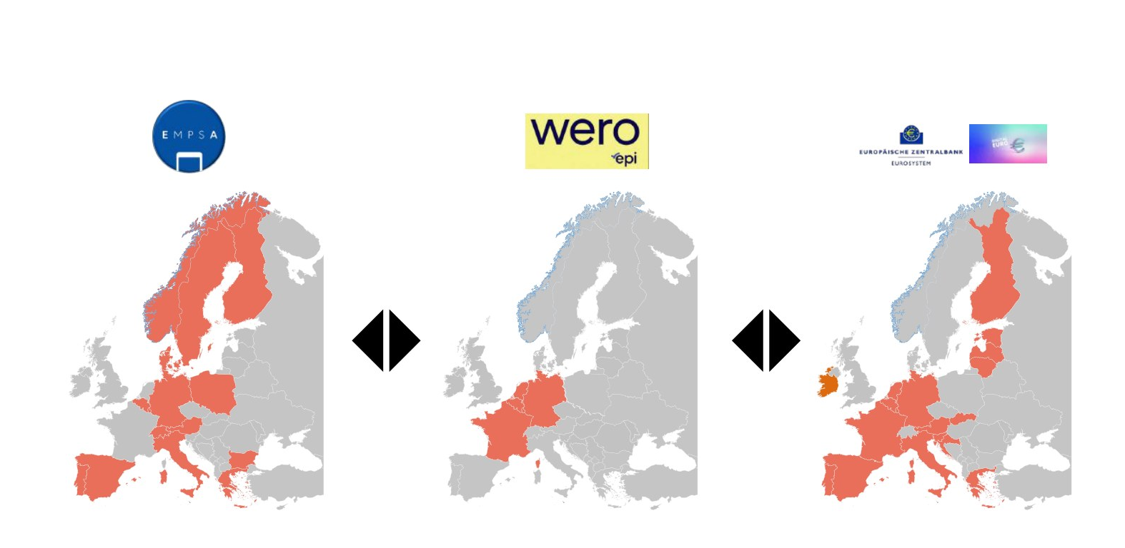
A geographic map can show participating countries or institutions without showing universal merchant acceptance. National person-to-person success does not automatically translate into cross-border e-commerce acceptance. The historical comparison of European initiatives illustrates how interoperability might extend reach, but actual usefulness depends on compatible rules, interfaces, merchant integration and commercial incentives. A payment system can be technically reachable while remaining unfamiliar to users.
Historical exits by bank, telecom and merchant payment projects demonstrate that access to customers or infrastructure does not guarantee a sustainable product. Examples include bank-led initiatives such as Paydirekt, telecom wallets and merchant-specific systems. Their causes should not be collapsed into one universal explanation: timing, governance, pricing, incumbent responses and customer experience differ. A discontinued project can also contribute technology or experience to a later service rather than representing a complete loss of learning.
Competition policy and payment regulation can influence these dynamics. Access to essential interfaces, portability, interoperability and rules against exclusion may lower entry barriers, but can also require careful governance and security standards. A subsidy that solves an initial coordination problem may be commercially rational, while perpetual subsidies with no credible positive contribution are not evidence of a viable network. The relevant welfare assessment includes consumer surplus, merchant costs, innovation, inclusion and resilience, rather than provider profit alone.
Public digital money and the rationale for a digital euro
The Libra proposal announced in 2019 showed why a global privately governed payment instrument could raise questions about monetary sovereignty, competition, governance and financial stability before achieving widespread use. Public authorities also investigate digital forms of central-bank money. A retail central-bank digital currency would give the public a digital claim on the central bank, distinct from a commercial-bank deposit or private stablecoin.
The proposed digital euro can be assessed against several objectives: continued access to public money as commerce becomes more digital, pan-European acceptance, resilience, privacy and reduced dependence on particular private infrastructures. These are policy objectives, not benefits established solely by announcing a project. Costs include building and maintaining infrastructure, customer support, fraud prevention, changes for merchants and intermediaries, and potential effects on bank funding.
Status checked on 14 October 2026: the ECB describes a twelve-month pilot expected to begin in the second half of 2027 and readiness for a potential first issuance during 2029, conditional on the necessary legislative framework and decisions. A planned pilot is not a launched retail currency, and its expected timetable is not a guarantee. The analysis below describes design proposals and mechanisms rather than claiming that the public can already use a digital euro.
Project status: ECB, Digital euro pilot.
Access, privacy, holding limits and conditional payments
A public digital payment instrument requires an operational distribution model. Intermediaries can provide onboarding, wallets and customer services even though the monetary claim is against the central bank. Online and offline modes have different information flows, fraud controls and recovery needs. Offline functionality can support resilience and privacy when connectivity fails, but secure devices, lost-value risks and synchronisation still require design choices.
| Dimension | Design objective or proposed mechanism | Economic trade-off |
|---|---|---|
| Monetary claim | Public central-bank money | Issuer safety does not remove cyber or service-provider risk. |
| Access | Intermediated services through applications, cards or other accessible interfaces | Usability must accommodate people with different devices and abilities. |
| Offline use | Payments without continuous internet access | Resilience and privacy must be balanced with device and fraud controls. |
| Privacy | Data minimisation with distinct online and offline arrangements | Pseudonymity, anonymity and lawful data access are different properties. |
| Holding limits | Limit use as a large-scale investment or flight-to-safety balance | Funding stability must be reconciled with convenient payments. |
| Remuneration | The proposed retail design is non-interest-bearing | Reduces incentives to replace savings deposits. |
| Linked-account funding | Automatic funding of payment shortfalls and transfer of excess receipts | Convenience depends on sufficient bank funds and reliable connections. |
| Conditional payments | Optional services such as payment on delivery | Useful automation still requires reliable information and dispute resolution. |
| Acceptance | Retail, online, person-to-person and relevant public-sector use cases | Common standards do not eliminate merchant integration costs. |
The ECB's proposed design distinguishes non-programmable money from optional conditional payment services and includes holding limits, no remuneration and linked-account funding mechanisms. No particular numerical holding limit should be treated as settled merely because a value has been examined in a technical exercise. Basic individual use is intended to be free, while providers can have costs and offer additional services. These design statements do not mean every participant or every value-added service would be free of charge.
Design description: ECB, FAQs on the digital euro, as checked on 14 October 2026.
Comparing a bank transfer with a digital-euro payment
In a conventional account-to-account transfer, the payer's bank deposit falls, the payee's bank deposit rises and any interbank obligation is settled through the relevant infrastructure, potentially in central-bank money. The customers continue to hold commercial-bank claims. In a digital-euro transfer, the customer's monetary balance would be a central-bank claim. Funding and defunding connect that balance with a linked bank account where used; the customer-facing intermediary remains distinct from the issuer of the money.
For a conceptual example, a person with EUR 30 of digital-euro balance wants to make an EUR 80 payment. If the design permits automatic linked-account funding and the account has sufficient available funds, EUR 50 can be drawn to cover the shortfall. Conversely, receipts above a holder's permitted balance can be transferred back to a linked bank account under a waterfall arrangement. This example illustrates the mechanism; it does not assume a particular final holding limit, fee or technical routing.
| Question | Instant bank-account transfer | Proposed digital-euro transfer |
|---|---|---|
| What does the customer hold? | A deposit claim on a commercial bank | A central-bank monetary claim accessed through the distribution arrangement |
| What changes between customers? | Bank deposit balances | Digital-euro balances, with funding or defunding where applicable |
| Where does settlement safety come from? | Bank payment arrangements and their settlement infrastructure | Public monetary claim and the digital-euro system's rules and controls |
| Is an internet connection always necessary? | Depends on the service and initiation channel | The proposed design includes a distinct offline mode |
| What remains necessary? | Authentication, compliance, fraud prevention and customer service | Authentication, appropriate compliance, fraud prevention and customer service |
| What is the main comparison? | Existing speed, reach, protections and total cost | Additional public-money access, reach and resilience relative to implementation and funding effects |
Adding funding and defunding steps can create operational dependencies, but a diagram with more arrows is not enough to prove that the service is inefficient. Some steps may be automated and the objective may include access to a different monetary claim or an offline mode. Equally, public issuance does not by itself establish that a new service improves every online transaction. The correct assessment identifies the particular use case, the benefits delivered and the complete resource and risk costs.
The same framework applies across payment innovation: identify the money, the service layers, the participants, the incentives and the counterfactual. Speed without acceptance has limited value; broad acceptance without reliable protection can harm users; profitability without competitive pressure can coexist with excessive merchant costs. A durable payment arrangement aligns these requirements sufficiently to attract repeated use and withstand operational and financial stress.
Appendix A. Formula Reference
This reference collects the main calculations used throughout the manual. Each identity must be read together with its measurement convention and assumptions. A stock measured at a reporting date is not interchangeable with an average stock over a year; a percentage of assets is not a percentage of deposits; an accounting value is not necessarily an immediately realisable market value. Worked applications and the economic reasoning behind the formulas remain in the relevant chapters.
Balance sheets, leverage and loss absorption
Let denote total assets, liabilities and equity, measured on a consistent accounting or valuation basis. The balance-sheet identity and two simple capital measures are:
If an asset loss is recognised immediately and liabilities remain unchanged, and . The percentage loss of equity is , while the new equity ratio is . Using the original asset denominator would produce a different measure. An institution with no additional loss absorbers exhausts its equity when ; it is therefore wiped out by an asset loss fraction . The regulatory leverage ratio uses a specific exposure measure and Tier 1 capital, so it is not simply the reciprocal of accounting leverage.
Profitability, margins and operating efficiency
Let be net income for a period and let bars indicate average balance-sheet stocks over that same period. Return on assets and return on equity satisfy:
The last equality requires the same net-income numerator and compatible average stocks. Higher leverage increases the sensitivity of shareholders' returns to profits and losses; it does not by itself improve the profitability of the underlying assets.
For interest income and interest expense , net interest income is . A conventional net interest margin is , where denotes average interest-earning assets. Some datasets instead divide by average total assets. The denominator must always be stated. A loan–deposit spread, , is a difference between two yields with different denominators; it is not automatically equal to NIM. Here is average lending and average deposits. The cost-to-income ratio is operating expenses divided by operating income under the stated accounting definition.
Present value, duration and interest-rate shocks
For deterministic cash flows discounted at a constant per-period yield , the price is . Macaulay duration measures the present-value-weighted payment date, while modified duration converts it into first-order price sensitivity:
This convention assumes one compounding period per unit of . Use a duration measure consistent with the yield and compounding convention. Enter a 150-basis-point yield change as , not . The approximation ignores convexity, changes in cash flows and nonparallel yield-curve movements. For material shocks, reprice the actual cash flows or add an appropriate convexity adjustment.
Expected credit loss and loan pricing
For one exposure and a specified horizon, probability of default , loss given default and exposure at default give the basic expected-loss calculation:
The recovery rate must use the same claim basis as EAD and should reflect the assumed timing and costs of recovery. This elementary product is not a complete accounting expected-credit-loss model: discounted cash-flow shortfalls, changes in exposure and multiple economic scenarios can matter.
A simple pricing decomposition adds funding cost, operating cost, expected loss and a target margin. An exact one-period break-even coupon requires explicit payoff assumptions. If a loan of principal pays when it performs and recovers in default, with default probability , funding rate and end-of-period costs , then:
The denominator matters because the coupon is not collected in default. Do not substitute this formula into an exercise that assumes a different recovery basis or simply defines an additive pricing convention. Expected profit, accounting provisions and unexpected-loss capital also measure different things.
Borrower participation and adverse selection
In a simple limited-liability model, a borrower receives principal and its project pays with probability , otherwise zero. If successful-project repayment is , the borrower's expected payoff is:
With a zero outside option and strict positive participation, . At equality the borrower is indifferent; whether it participates must be specified. If the types that remain in the market change when the rate passes a threshold, expected repayment is piecewise. A higher promised interest rate can then lower expected bank revenue by driving safer borrowers out of the pool.
Securitisation and tranche losses
Let total pool loss , tranche attachment point and detachment point use the same units, with . The amount of loss allocated to the tranche and the fraction of its principal lost are:
For a tranche covering pool losses from 5% to 15%, a 9% pool loss consumes four percentage points of pool principal, equal to 40% of that tranche. It is not a 4% loss of the tranche itself. This static waterfall ignores the timing of interest and principal, fees, triggers and recoveries; a transaction model must follow its actual contractual rules.
Liquidity insurance and expected utility
Suppose a fraction of savers needs early consumption and the remaining fraction consumes later. If one unit retained until the later date yields and early liquidation yields one, the basic resource constraint per initial saver is:
where is initial wealth. When and , the interior optimum satisfies , or , together with the binding resource constraint. Boundary and incentive constraints must also be checked. An allocation can improve on autarky without being the exact optimum.
For a risky withdrawal payoff , expected utility is . With concave utility it generally differs from . In particular, the late-consumer utility from a run lottery is , not . This distinction is essential when comparing withdrawal with waiting.
Run capacity, insurance and liquidation
If liquid resources total and each early claimant is promised , the number paid in full is , with residual resources . The residual claimant's payment must be included when calculating expected utility under a random queue. A guarantee of principal does not necessarily eliminate an incentive to withdraw when the immediate contractual payment is greater than .
If a redemption needs cash , immediately available liquid assets are , and securities sell at haircut relative to book value, the book value that must be sold is:
These expressions assume enough saleable assets exist and that the haircut is constant. The loss is larger than simply multiplying the cash shortfall by , because the sale must raise the full shortfall after the discount.
Capital and liquidity regulation
Under a simplified standardised credit-risk calculation, risk-weighted assets are , where is the applicable risk weight. A capital ratio is the specified eligible capital divided by RWA, for example . Actual regulatory RWA can also include market risk, operational risk and adjustments. The unweighted leverage ratio divides eligible Tier 1 capital by the regulatory exposure measure, which can include off-balance-sheet items.
Two complementary liquidity measures are:
Eligibility, valuation haircuts, inflow caps and funding weights are part of the definitions. The ratios should not be calculated by inserting arbitrary balance-sheet categories. Capital absorbs losses; liquidity resources meet payments. Passing one ratio does not prove that all solvency, funding or concentration risks are controlled. The regulation chapter explains the applicable standards and historical examples.
Money stocks, payments and the money multiplier
In a stylised system, let currency held by the public be , deposits be and bank reserves be . Broad money in this simplified definition is ; the monetary base is . Writing and yields the accounting relationship:
This identity is not a mechanical causal rule by which central-bank reserves determine bank lending. Currency preferences, reserve holdings, loan demand, funding costs and monetary-policy implementation all matter. Nor does this stylised reproduce every official monetary aggregate. Loan origination creates a loan asset and a matching deposit liability; repayment of principal destroys those two claims. Payment to another bank changes the distribution of deposits and reserves across banks rather than necessarily changing their system-wide totals.
Stablecoin backing and payment business economics
A simple stablecoin backing ratio is market value of reserve assets divided by redeemable token liabilities, measured at the same date and on the same valuation basis. A ratio of at least one does not by itself guarantee immediate redemption: custody, legal priority, settlement, liquidity and operational arrangements remain essential. A discount to the reference unit is , where is the observed token price and the promised reference value.
For a payment business processing transactions, earning average revenue and incurring variable cost per transaction, contribution before fixed costs is . With fixed cost and positive unit contribution, operating break-even volume is . Transaction counts, payment values and fees as a percentage of value are distinct units; a model that mixes them will not reconcile. Customer balances held in a closed-loop system are also not automatically accounting revenue or profit.
Appendix B. Glossary
The definitions below provide a quick route back into the concepts used in the chapters. They distinguish economic mechanisms, accounting measures and regulatory categories rather than treating similar-sounding terms as synonyms.
Intermediation, information and contracts
- Adverse selection
- An information problem before contracting in which counterparties differ in characteristics that the other party cannot fully observe. Contract terms can change the mix of applicants that participate.
- Agency relationship
- An arrangement in which one party acts for another. Divergent objectives and incomplete observation can create costs that incentives, monitoring and contractual restrictions try to contain.
- Asset transformation
- The process of acquiring assets with one set of risk, maturity, liquidity, size or currency characteristics and issuing claims with another. The transformation reallocates risk and can create new vulnerabilities.
- Asymmetric information
- A situation in which parties to a transaction possess different relevant information. Adverse selection and moral hazard concern different timings and forms of this problem.
- Broker
- An intermediary acting as an agent to arrange transactions. A dealer instead trades as principal and holds the resulting position on its own balance sheet.
- Collateral
- An asset or right securing an obligation and available to a creditor under the contract and applicable law. Its value depends on enforceability, priority, sale costs and conditions at recovery.
- Commitment
- A lender's contractual promise to provide funds subject to stated conditions. A commitment can create liquidity exposure before it becomes a drawn loan.
- Consumption smoothing
- Using saving, borrowing and insurance to transfer consumption across time or states of the world, subject to an intertemporal resource constraint.
- Covenant
- A contractual obligation or restriction, such as a reporting requirement or leverage limit. Breach can give creditors rights to renegotiate, suspend advances or accelerate repayment.
- Credit rationing
- A situation in which borrowers willing to accept the prevailing terms cannot obtain all the credit they demand. Information and incentive effects can prevent a higher interest rate from clearing the market.
- Delegated monitoring
- Having an intermediary monitor borrowers on behalf of multiple investors, potentially avoiding duplicated effort while creating a separate need to discipline the intermediary.
- Direct finance
- Funding in which the ultimate investor holds a claim issued by the ultimate borrower, even if an intermediary arranges or distributes it.
- Indirect finance
- Funding through an intermediary that holds a claim on a borrower and issues a distinct claim to its own funders.
- Limited liability
- A legal or model feature limiting an investor's losses to a defined stake. The precise liability of a borrower or guarantor depends on the contract and law.
- Moral hazard
- An incentive problem after contracting when a party can take actions that another party cannot fully observe or control and some consequences are borne by others.
- Relationship lending
- Lending based partly on information accumulated through repeated interaction, account activity and borrower contact. It can improve screening while increasing switching costs.
- Screening
- Gathering and assessing information before a transaction to distinguish borrower quality, investment prospects or counterparty suitability.
- Seniority
- A claim's priority relative to other claims in receiving payment or bearing losses. Seniority is different from the probability that the debtor enters default.
- Syndicated loan
- A loan provided by multiple lenders under a coordinated contractual arrangement, often with an arranger and an administrative agent.
Accounts, valuation and credit risk
- Assets
- Resources and claims recognised on an institution's balance sheet, including loans, securities and cash. Book value, market value and liquidation proceeds can differ.
- Cost-to-income ratio
- Operating expenses divided by operating income under a stated definition. Differences in classification and exceptional items affect comparisons.
- Credit spread
- A yield difference relative to a specified benchmark. It can compensate for expected loss, unexpected risk, liquidity and other factors rather than default risk alone.
- Duration
- A measure related to the timing of discounted cash flows and their sensitivity to yield changes. Modified duration provides a local approximation to percentage price changes.
- Equity
- The residual interest after liabilities are deducted from assets. Equity absorbs losses before creditors under the relevant accounting and legal framework.
- Expected loss
- The probability-weighted average credit loss over a specified horizon. A basic exposure-level approximation multiplies default probability, loss given default and exposure at default.
- Exposure at default (EAD)
- The amount exposed when a debtor defaults, potentially including future drawings on committed facilities and other contract-specific items.
- Haircut
- A reduction applied to an asset's reference value for collateral, prudential or sale purposes. The haircut's meaning and valuation base must be stated.
- Impairment allowance
- An accounting adjustment for expected or identified credit losses under the relevant reporting framework. Recognising an expense need not mean that a payment default has already occurred.
- Leverage
- The relationship between an institution's exposures or assets and its capital. Greater leverage magnifies shareholders' sensitivity to asset-value changes.
- Liabilities
- Obligations owed to other parties, such as deposits, debt securities and borrowing. The timing and conditions of payment determine their funding and liquidity implications.
- Loss given default (LGD)
- The fraction of exposure lost conditional on default, after allowing for the assumed recovery process and costs.
- Mark-to-market
- Valuation using current market prices or appropriate market-based estimates. Economic value changes may be relevant even when accounting recognition follows another convention.
- Net interest income
- Interest income less interest expense over a period. It is an amount, while a net interest margin is that amount divided by a specified asset base.
- Nonperforming loan (NPL)
- A loan meeting a defined nonperformance criterion, commonly involving material arrears or unlikeliness to pay. Exact definitions differ across reporting and regulatory frameworks.
- Probability of default (PD)
- The probability of entering a defined default state during a specified horizon. A lifetime PD and a one-year PD are not interchangeable.
- Recovery rate
- The recovered fraction of a specified claim, measured under stated timing, discounting and cost assumptions.
- Return on assets (ROA)
- Net income divided by assets, often average assets over the income period. It measures profitability relative to the asset base.
- Return on equity (ROE)
- Net income divided by equity, often average equity. Leverage can increase ROE while also increasing risk.
- Write-off
- Removal of all or part of a recognised asset when recovery is no longer reasonably expected under the applicable accounting policy. It differs from an earlier impairment allowance.
Funding, crises and safeguards
- Bank run
- A rapid attempt by many creditors or depositors to withdraw or refuse renewal. The expectation that others will withdraw can make early withdrawal individually attractive.
- Bridge loan
- Temporary financing intended to cover a period before longer-term funding or another anticipated cash inflow becomes available. It need not be a revolving facility.
- Capital buffer
- Loss-absorbing resources held above a defined minimum or internal requirement. It is not the same thing as a stock of cash available for withdrawals.
- Contagion
- Transmission of distress across institutions or markets through contractual exposures, common assets, information, confidence or funding channels.
- Deposit insurance
- A scheme protecting eligible depositors within defined coverage limits and conditions. Coverage of principal does not automatically cover every promised interest payment or every type of claim.
- Deposit franchise
- The economic value associated with a bank's ability to attract and retain deposits on advantageous terms, allowing for servicing costs, customer behaviour and competition.
- Fire sale
- A sale driven by urgent funding needs at a price depressed by limited buyer capacity or market illiquidity. Such sales can transmit losses to other holders of similar assets.
- Funding liquidity
- The ability to obtain cash or other immediately usable means of payment to meet obligations when due.
- High-quality liquid assets (HQLA)
- Assets satisfying the eligibility and valuation conditions of a liquidity framework. Their role is to provide reliable resources under stress.
- Illiquidity
- Inability to meet payments on time using available funds or reasonable funding options, even where ultimate asset values may exceed liabilities.
- Insolvency
- A condition in which an institution cannot meet the applicable solvency test, often associated economically with asset values below liabilities. Legal definitions depend on jurisdiction.
- Lender of last resort
- A central bank or other designated institution providing emergency liquidity under specified conditions when ordinary funding channels fail.
- Liquidity coverage ratio (LCR)
- A regulatory ratio comparing eligible liquid assets with stressed net cash outflows over a 30-day horizon, using prescribed definitions and adjustments.
- Maturity transformation
- Funding longer-lived assets with claims that mature or can be withdrawn earlier. The resulting renewal and liquidity risks require active management.
- Net stable funding ratio (NSFR)
- A regulatory measure comparing available stable funding with the required stable funding of assets and activities over a longer horizon.
- Refinancing risk
- The risk that maturing obligations cannot be replaced on feasible terms, even when the underlying project or asset has not reached its final cash-flow date.
- Resolution
- A framework for handling a failing financial institution while pursuing defined public objectives, potentially including continuity of critical functions and allocation of losses to investors.
- Risk-weighted assets (RWA)
- A regulatory exposure measure incorporating specified risk weights or model-based requirements. It is not the accounting total of assets.
- Systemic risk
- The risk of financial disruption with consequences for the functioning of the broader system and the real economy, including amplification through interconnected institutions and common exposures.
Markets, money and payments
- Asset-backed security (ABS)
- A security whose payments depend on an underlying pool of financial assets, subject to the transaction's legal structure and payment rules.
- Attachment and detachment points
- The pool-loss thresholds at which a tranche begins to absorb losses and becomes fully exhausted.
- Broad money
- A monetary aggregate including currency and specified deposit-like instruments held by designated sectors. Its composition depends on the statistical definition used.
- Central bank digital currency (CBDC)
- A digital monetary liability of a central bank designed for a defined group of users and payment functions. Retail and wholesale proposals differ in access and purpose.
- Clearing
- Processing and reconciling transaction instructions and determining the resulting obligations before final settlement.
- Closed-loop balance
- A prepaid balance usable within a defined merchant or platform network, rather than general-purpose money accepted everywhere.
- Correspondent banking
- An arrangement in which one bank provides payment, account or other services to another, often across borders.
- Credit creation
- Expansion of loan claims and associated obligations. A bank loan commonly creates a deposit at origination, while subsequent payments require settlement and funding management.
- Custody
- Safekeeping and administration of assets and records on behalf of clients, with appropriate segregation and ownership controls.
- Digital wallet
- An interface or arrangement for storing payment credentials, accessing account balances or controlling digital assets. Its economic and legal functions depend on what it actually holds or accesses.
- Interchange fee
- A payment between participating institutions within a card arrangement under its rules. It differs from the total fee a merchant pays its payment provider.
- Investment banking
- Activities including securities issuance, underwriting, capital-raising advice and mergers-and-acquisitions services. Different activities involve different agency and principal risks.
- Market liquidity
- The ability to trade an asset promptly in meaningful size without an excessive price concession. It can deteriorate precisely when many holders need cash.
- Monetary base
- Central-bank monetary liabilities included in the chosen definition, commonly currency and bank reserves. It differs from broad money held by the public.
- Money destruction
- Reduction of monetary claims, such as when repayment of bank-loan principal cancels a deposit liability and the corresponding loan asset.
- Network effects
- Changes in the value of a service as the number or composition of its users changes. Payment platforms can link adoption on the customer side to acceptance on the merchant side.
- Quantitative easing (QE)
- Central-bank asset purchases used for monetary-policy purposes. Their balance-sheet effects depend on the seller and settlement chain; reserves are not mechanically lent onward to households.
- Redemption
- Exchanging a financial claim for the assets or money promised under its terms. Legal entitlement and practical access are as important as the issuer's stated backing.
- Reserves
- In monetary accounting, bank balances at the central bank used for settlement and other permitted purposes. Stablecoin reserve assets are a different category and should not be confused with central-bank reserves.
- Securitisation
- Financing or risk transfer using securities linked to a pool of exposures, often with different priorities and loss-bearing tranches.
- Settlement
- Discharge of a payment or securities obligation through the final transfer of the required asset, subject to the relevant system's rules and legal finality.
- Special-purpose vehicle (SPV)
- An entity established for a defined transaction or activity, frequently used to hold securitised assets. Legal separation and risk transfer depend on the actual structure.
- Stablecoin
- A crypto-asset designed to maintain a stable value relative to a reference asset or unit. A target value does not guarantee that market prices or redemption proceeds always equal it.
- Tokenisation
- Representing claims or assets in digital-token form within a specified infrastructure. It does not by itself change the underlying economic claim, legal priority or credit risk.
- Tranche
- A class of claims with a defined position in a payment or loss waterfall. A senior tranche can remain exposed to correlated or sufficiently severe pool losses.
- Underwriting
- Assessment and assumption of defined risks in lending, insurance or securities issuance. In an issuance, the underwriter's commitment determines how much placement risk it bears.