
1. Foundations, scope and modelling strategy
Introduction
Business-cycle macroeconomics asks why aggregate production, employment, consumption and investment move together, which mechanisms propagate disturbances across periods, and whether public policy can improve economic outcomes. The objective is not to memorize a single diagram or policy prescription but to understand how internally consistent models turn economic assumptions into quantitative predictions.
A useful model specifies exogenous drivers, endogenous decisions, constraints, markets and an equilibrium concept. The Dynamic Stochastic General Equilibrium (DSGE) methodology adds decisions across time, random disturbances and mutually compatible markets. Its value is not that every assumption is literally true; its value is that explicit assumptions make a model testable and criticizable.
The development proceeds from empirical targets to firms' factor demand and households' intertemporal choices. It then establishes the equilibrium system, chooses parameter values, approximates the model locally, solves the resulting dynamics and compares the quantitative predictions with observed business cycles.
Integrated theoretical explanation
Macroeconomics studies the decisions and constraints that jointly determine production, employment, spending and prices. Business-cycle theory focuses on deviations in these quantities around their longer-run paths and, above all, on why fluctuations spread across markets and persist over time. An expansion in output can coincide with higher employment, private spending and investment even though the sectors of the economy are connected by very different mechanisms. A satisfactory model therefore needs more than an accounting relation: it must specify who makes choices, which trade-offs they face, what information they use, and how market-wide outcomes are determined.
The distinction between explaining an observed correlation and predicting the effect of a deliberate intervention is essential. Two variables may move together because both respond to an omitted factor. Raising public spending, changing the tax system or setting a different interest-rate rule alters the decision environment itself. To evaluate such counterfactuals, a model should identify the behavior that generates aggregate relationships rather than assuming that a historical empirical association will survive a change in policy. This is why economists separate positive questions about what happens from normative questions about what policy ought to do, which additionally require an explicit welfare criterion.
A model is intentionally selective. The economy contains more goods, agents, contracts and institutions than a tractable mathematical representation can describe. Abstraction becomes productive when it removes details irrelevant to a given question while preserving the mechanism that matters. An elegant model can be unsuitable for a particular question: one without intertemporal saving cannot explain long-run capital accumulation, whereas a model without nominal variables cannot directly determine inflation or the nominal impact of central-bank actions. The proper standard is therefore not maximum complexity, but transparent assumptions, internal consistency and an empirically meaningful purpose.
Endogenous variables are determined jointly within the system; exogenous variables enter from outside it. In the benchmark Real Business Cycle framework, labor hours, output, consumption and the capital stock are endogenous, while the exogenous productivity innovation follows a specified stochastic process. This classification depends on the model, not on a permanent property of the variable. Tax revenue may be a mechanically endogenous share of income, whereas the statutory tax rate may be an exogenous policy instrument. Calling something exogenous does not establish that it is unimportant: it identifies the boundary of the explanation that the model currently offers.
The word dynamic means that decisions made at one date have consequences at later dates. Capital accumulated today is productive tomorrow; expected future returns affect saving today; and a shock may have effects well after the initial disturbance. Stochastic means that at least some future outcomes are uncertain and that new information arrives over time. General equilibrium requires that the choices of different agents and the quantities exchanged in different markets be jointly compatible. Together these features give the DSGE methodology its structure: specify preferences and production opportunities, derive optimal choices, determine market clearing and characterize how equilibrium responds to random disturbances.
Real Business Cycle theory established a disciplined use of intertemporal optimizing models for quantitative macroeconomics. It emphasizes real disturbances, especially productivity, and examines whether their propagation through consumption smoothing, labor allocation and capital accumulation can produce observed business-cycle movements. That is a methodological contribution independent of whether technology shocks alone explain every recession. The same strategy of deriving behavior from explicit optimization also underlies later models that add nominal rigidities, monetary policy and financial frictions. Those extensions are distinct from the RBC system derived in this volume.
Formal framework and essential relationships
Accounting versus behavior
The expenditure identity is true by definition at the aggregate level. By itself it does not determine the behavior of C, I, or policy; equilibrium models add decision rules and resource restrictions.
Endogenous versus exogenous variables
Deciding what is inside a model is a research choice. A technology innovation is exogenous in the baseline RBC environment, while consumption, capital accumulation and employment emerge endogenously.
DSGE interpretation
Dynamic · Stochastic · General equilibrium
A model can be dynamic without being stochastic, or stochastic without achieving market clearing. In a DSGE model the three features are combined and calibrated or estimated to connect shocks with data.
Explanations, derivations and empirical applications
The questions addressed by business-cycle theory
The essential questions concern the causes of aggregate fluctuations, the scope for policy intervention and the contribution of structural economic models. Answers depend on the mechanism being considered and the evidence available.
Macroeconomic Questions
Business-cycle analysis is organized around several distinct questions. We need to explain the causes of cyclical movements and understand how prices respond during expansions and recessions. We also need to distinguish what economic policy can accomplish under a specified model from what it should accomplish once the relevant welfare objective is stated. Monetary policy is a particularly important application, but its analysis requires a model with the appropriate nominal features.
Answers
A quantitative approach combines empirical measurement with economic theory. The starting point is a careful account of aggregate facts; the next step is to identify mechanisms capable of generating those facts consistently. Models become useful when they yield testable quantitative answers rather than just verbal stories. This dialogue between formal explanation and observed outcomes is the central research method developed throughout this volume.
A Method Rather Than A Doctrine
Keynes described economic theory as a method of disciplined reasoning rather than a collection of policy conclusions directly applicable without analysis. The value of theory lies in making assumptions and implications explicit.
What Is A Model?
The role of a model is to make its economic assumptions explicit and identify the particular outcomes to be explained. A useful representation organizes complex interactions into a tractable system whose predictions can be compared with the facts.
A model is a compact representation of a theory, constructed to organize economic reasoning. Precisely because it abstracts from the full complexity of the economy, its usefulness depends on how well the retained assumptions capture the mechanism of interest. It should generate interpretable implications that can be confronted with data, rather than claim to reproduce every institutional or behavioral detail.
Why Do We Need Models?
Thomas J. Sargent compares economic inference to learning the rules of a game by observing its play. Economic policy adds a complication: interventions can change the rules themselves. Detecting historical patterns is therefore insufficient for predicting responses to new policy regimes; structural models must explain how decisions respond to the altered environment.
How Can Models Help Us?
A set of explicit macroeconomic models helps organize competing explanations by identifying the mechanisms, state variables and constraints that each explanation requires. The discipline comes from connecting verbal claims to a coherent model and confronting its predictions with evidence.
Which Model Is The Right One?
Choose a model whose mechanisms match the question. Household choices require an explicit treatment of preferences and constraints; dynamic questions require decisions across dates. The model should reproduce the relevant empirical facts while abstracting from details that do not affect the mechanism under study.
Model = Device Of Help
A model is useful only relative to a question. A local street map and an international transport map represent different features because they support different decisions. Economic models likewise retain the mechanisms relevant to the question being studied.
Endogenous Or Exogenous?
An exogenous variable is treated as a model input whose law of motion is specified independently of the endogenous decisions under study. An endogenous variable is a model outcome, pinned down by equilibrium conditions. In the RBC framework productivity innovations are imposed from outside, whereas labor supply, investment and consumption are determined by households and firms. The same quantity can play a different role in another model, depending on the research question.
DSGE Models
DSGE denotes dynamic, stochastic, general-equilibrium modelling. Dynamic decisions link successive periods; stochastic shocks represent information that is not known in advance; and general equilibrium requires the behavior of different agents and markets to be mutually consistent. The methodology encompasses RBC models and New Keynesian models. Its formal discipline is especially relevant for studying whether the behavior that generates macroeconomic outcomes changes when policies or incentives change.
Real Business Cycle Models
A time series can be represented as a long-run trend plus a cyclical component, although the split is not uniquely observable. A deterministic linear trend assumes a constant average growth rate; the Hodrick–Prescott procedure chooses a smooth changing trend by penalizing second differences. Results depend on the smoothing parameter and on end-point behavior, so filter choice must be stated explicitly.
The RBC approach is associated with the influential contributions of Kydland and Prescott. It replaces ad hoc aggregate behavioral rules with conditions derived from agents’ intertemporal optimization and seeks a quantitative account of output, hours, investment and consumption fluctuations. Productivity innovations provide the benchmark driving disturbance. The empirical question is whether these disturbances, transmitted through equilibrium labor and capital decisions, reproduce the characteristic movements observed in the data.
Microfoundations - Saving & Investment
In the Solow model a fixed share of output is saved. With constant population, per-worker capital obeys the same accumulation equation as aggregate capital.
The saving rate is imposed rather than chosen by optimizing households. Population growth requires an additional normalization factor.
The linear consumption rule relates demand to disposable income:
Here c₀ is autonomous consumption and c₁ is the marginal propensity to consume. A structural model derives consumption from preferences and constraints instead of treating these coefficients as policy-invariant.
Readings
Further reading includes Robert G. King and Sergio T. Rebelo, “Resuscitating Real Business Cycles,” Handbook of Macroeconomics, Vol. 1B; George McCandless, The ABCs of RBCs; Carl E. Walsh, Monetary Theory and Policy; and Jordi Galí, Monetary Policy, Inflation, and the Business Cycle.
Prerequisites and study approach
The analysis assumes familiarity with supply and demand, consumption, investment and taxation; marginal utility and marginal rates of substitution; and constrained optimization, sums and logarithms. Infinite-horizon optimization extends these tools to decisions across time. Each equation should be read as an economic trade-off, with attention to its assumptions, timing and units.
Learning objectives
Develop the methods of dynamic macroeconomics through the RBC model; understand how productivity, intertemporal choices and equilibrium markets generate aggregate fluctuations; and evaluate the quantitative strengths and limitations of structural business-cycle models.
Summary of the economic argument
models are ways of organising our thoughts
Models that match relevant empirical facts can serve as laboratories for carefully specified economic counterfactuals.
The RBC model is a dynamic stochastic general-equilibrium framework for explaining business cycles.
the RBC model microfounds saving/investment behaviour
Synthesis
A structural model is a device for answering explicit questions, and good models must be judged against the relevant facts and policy counterfactuals.
2. From traditional macroeconomics to microfoundations
Introduction
The central reason for microfoundations is that a reduced-form rule need not remain stable when policy changes. In a simple Keynesian-cross exercise, consumption responds mechanically to disposable income; in a structural model, the same behavior derives from a household choosing consumption, saving and labor while respecting an intertemporal budget constraint.
The familiar IS–LM framework provides an intuitive description of short-run policy transmission, but its behavioral coefficients and schedules are not a complete theory of individual choice. A change in tax policy or interest-rate expectations may also change the very behavior encoded in those schedules. Microfoundations make those responses explicit by considering preferences, incentives, technologies and information.
The Solow growth model motivates capital accumulation, constant returns to scale and balanced growth. Its saving rate is exogenous, however. An RBC model preserves physical capital accumulation while making consumption, saving and labor supply optimal choices, thereby linking growth-accounting logic to business-cycle propagation.
Integrated theoretical explanation
In a short-run expenditure model, national output is measured by the value of final goods and services produced, while aggregate expenditure is the sum of consumption, investment, government purchases and net exports. For a closed economy, equilibrium in the goods market requires planned spending to equal production. If consumption follows C = c₀ + c₁(Y − T), the marginal propensity to consume c₁ creates a feedback mechanism: additional autonomous demand raises income, some of that income is spent again, and equilibrium output changes by more than the initial demand impulse. This textbook multiplier depends on fixed prices, spare productive capacity and the assumption that the consumption rule does not itself change in response to policy.
The multiplier can be derived directly by collecting income terms. With lump-sum taxes, Y = c₀ + c₁(Y − T) + Ī + G gives (1 − c₁)Y = c₀ − c₁T + Ī + G. Therefore a one-unit increase in government purchases raises equilibrium income by 1/(1 − c₁) units when all other terms are held fixed. If income taxation is proportional, T = tY, the feedback from income to consumption is smaller and the corresponding expression becomes 1/[1 − c₁(1 − t)]. The difference illustrates automatic stabilization: taxes partially offset income movements without the need for a new discretionary fiscal decision.
The IS–LM description adds the interest rate and the money market to the basic goods-market equilibrium. The IS schedule collects combinations of income and the interest rate that are compatible with goods-market equilibrium, taking account of interest-sensitive expenditure. The LM schedule collects combinations that satisfy money demand and money supply at a given price level. A tax increase or fall in spending typically shifts IS to the left, while expansionary monetary policy shifts the LM schedule in the direction associated with lower interest rates at given income. The intersection provides an intuitive joint-equilibrium picture, but changes in expectations, labor supply or saving preferences are not fully explained by the reduced-form curves themselves.
The labor–leisure choice clarifies what is absent from a purely demand-driven representation. A household has a limited time endowment; working more hours produces wage income but leaves less leisure. A consumption–leisure indifference curve describes combinations delivering the same utility, while the budget line translates the wage into the amount of consumption that can be purchased by sacrificing leisure. At an interior optimum, the marginal rate of substitution equals the wage, expressed in appropriate consumption units. A change in taxes on labor income changes this relative price and therefore influences labor supply, which in turn alters aggregate production and the resources available for consumption.
A rise in the real wage has potentially competing effects. Through substitution, leisure becomes more expensive and work becomes more attractive. Through income, a richer household may choose to consume more leisure. Which effect dominates depends on preferences and the context of the wage change. For this reason, a model that assumes fixed labor supply cannot reliably answer every question concerning taxation or productivity. Introducing a utility-based labor supply decision allows the model to distinguish the incentive channel from the income channel and to examine the net outcome in equilibrium with firms' labor demand.
The Solow model supplies the other essential foundation: intertemporal capital accumulation. Output is produced from capital and effective labor, and a fixed fraction of output is invested. The investment rule and capital accumulation identity determine the evolution of productive capacity. When technology and population grow, dividing output and capital by effective labor converts a balanced growth path into a stationary representation. In that normalized economy, investment per effective worker must cover both physical depreciation and the dilution resulting from more effective labor. A stationary capital intensity can therefore coexist with continuing growth in aggregate capital and output.
The saving rule I = sY is useful for understanding transition dynamics but is not an optimal decision derived from household preferences. In a microfounded RBC model, households choose how much to consume and invest after considering future returns and the utility of consumption at different dates. The technology and accumulation equations survive, but the behavioral equation governing saving changes fundamentally. This transition is the intellectual bridge from introductory macroeconomic diagrams to the structural business-cycle model developed later in this volume.
Formal framework and essential relationships
Keynesian-cross benchmark and the fiscal multiplier
Consumption combines autonomous spending c₀ and a fraction c₁ of disposable income; Ī is exogenous planned investment. Goods-market equilibrium requires production Y to match demand.
An increase in government expenditure becomes income, which induces additional consumption and subsequent production. Under the model’s assumptions, each round is c₁ of the previous one.
A proportional income tax makes disposable income respond less than one-for-one to production. The tax rate t reduces the multiplier and acts as an automatic stabilizer.
Capital accumulation and balanced growth
With labor-augmenting technology A and workers L, dividing output and capital by AL produces variables per effective worker, which can converge to constant steady-state values even when aggregates continue to grow.
This discrete-time effective-worker equation is valid when A and L grow at rates μ and ν and I = sY. It makes the distinction between physical depreciation and dilution by effective-labor growth explicit.
Explanations, derivations and empirical applications
GDP And Demand
A reduced-form relationship gives a useful description of equilibrium under its assumptions. Deriving the underlying choices from household and firm optimization makes it possible to analyze how the relationship responds when policy or incentives change.
National expenditure is composed of consumption, investment, government spending and net exports, so Y = C + I + G + X − IM. In a simple closed economy, net exports disappear and consumption is specified as an increasing linear function of disposable income, C = c₀ + c₁(Y − T). Planned investment is taken as exogenous and the fiscal authorities choose taxes and public purchases. If taxes are proportional to income, T = tY, this creates an automatic stabilizer because a rise in production increases tax revenue and reduces the marginal feedback into private consumption.
Equilibrium On The Goods Market
Fit to text
Scroll horizontally to inspect the labels and values.
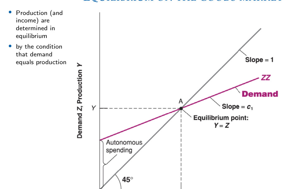
The Keynesian cross determines goods-market equilibrium where planned expenditure intersects the 45-degree line. At the intersection, planned spending equals output. The slope of the expenditure line is the marginal propensity to consume when taxes and investment are fixed.
Government Spending Multiplier
Fit to text
Scroll horizontally to inspect the labels and values.
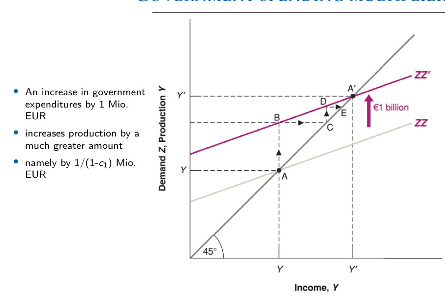
An increase in autonomous government spending shifts planned expenditure upward. Successive rounds of consumption raise equilibrium output by more than the initial expenditure change when the marginal propensity to consume lies between zero and one.
Is-Lm Model
Fit to text
Scroll horizontally to inspect the labels and values.
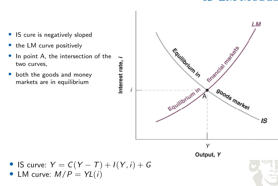
The IS curve represents goods-market equilibrium and slopes downward because higher interest rates reduce interest-sensitive spending. The LM curve represents money-market equilibrium. Their intersection jointly determines output and the interest rate.
Fiscal Policy
Fit to text
Scroll horizontally to inspect the labels and values.
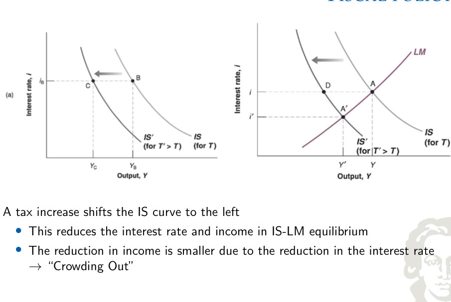
Higher taxes shift the IS curve left by reducing disposable income and consumption. With an unchanged LM curve, both output and the interest rate fall; the lower interest rate partially offsets the contraction by supporting investment.
Monetary Policy
Fit to text
Scroll horizontally to inspect the labels and values.
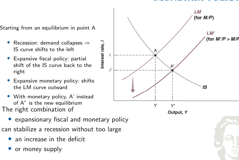
An increase in the real money supply shifts the LM curve outward. The lower equilibrium interest rate supports expenditure and output. Fiscal and monetary adjustments can therefore interact when stabilizing a decline in private demand.
Not All Taxes Are Created Equal
Lump-sum taxes and income taxes do not have identical implications. Changing a fixed tax payment shifts disposable income at every level of production. Changing the marginal income-tax rate also changes the slope of the household’s disposable-income schedule and the strength of the expenditure multiplier. A fuller analysis must additionally account for changes in the relative return to working, which affect the household’s optimal labor–leisure choice.
Consumption and leisure preferences
Fit to text
Scroll horizontally to inspect the labels and values.
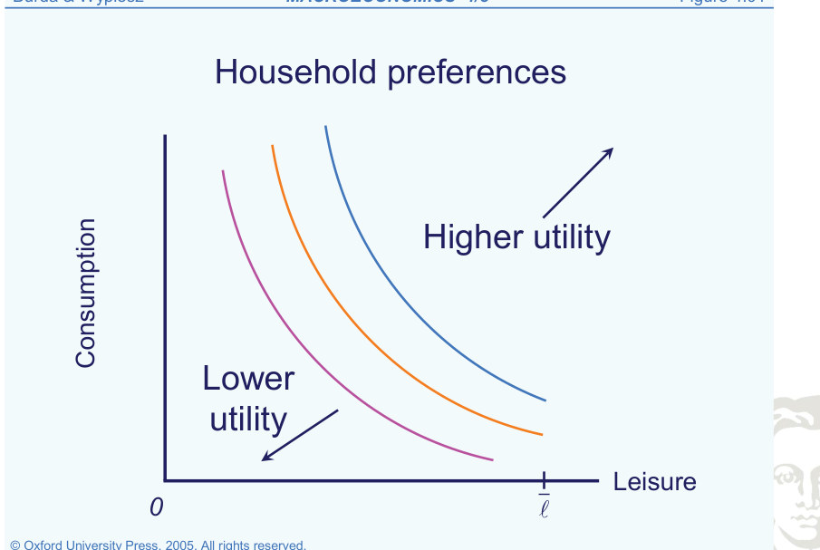
The consumption–leisure indifference curve
Fit to text
Scroll horizontally to inspect the labels and values.
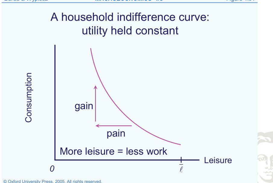
Interpreting household preferences
An indifference curve slopes downward because more leisure must be offset by less consumption to leave utility unchanged. Its slope gives the marginal rate of substitution. Curvature means the willingness to trade leisure for consumption changes across bundles. A higher indifference curve represents greater utility.
The household budget constraint
Fit to text
Scroll horizontally to inspect the labels and values.
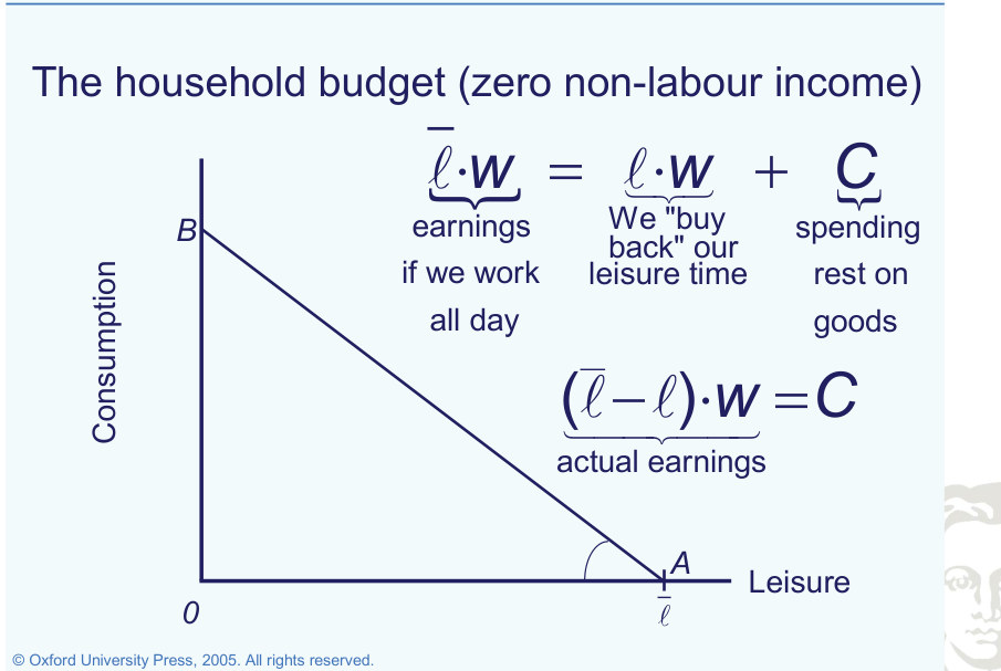
Choosing an attainable consumption–leisure bundle
Fit to text
Scroll horizontally to inspect the labels and values.
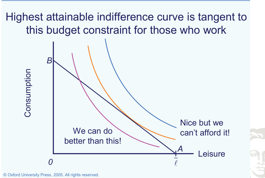
Optimal consumption and leisure
Fit to text
Scroll horizontally to inspect the labels and values.
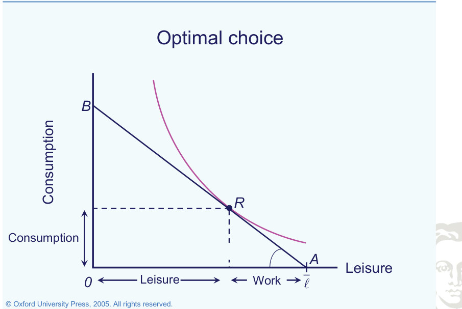
General Equilibrium?
The labor–leisure decision cannot be analyzed in isolation from production. If households prefer more leisure, firms receive less labor input, aggregate output changes and the economy’s feasible consumption possibilities also change. The same feedback operates in reverse when work becomes more attractive. A general-equilibrium analysis incorporates these mutually dependent adjustments rather than shifting one household budget line while leaving all aggregate factor-market conditions unchanged.
Production Function
The Solow production technology combines capital K, labor L and labor-augmenting productivity A, typically through Y = K^θ(AL)^(1−θ). The exponents determine marginal-product elasticities, and their sum of one gives constant returns to scale in the two productive inputs. A rise in A increases effective labor for a given number of workers; capital deepening and technological progress then jointly determine output per worker.
What Do ’Constant Returns To Scale’ Mean?
Constant returns to scale describe a proportional experiment in which every physical input increases by the same factor. With Cobb–Douglas exponents θ and 1 − θ, multiplying both capital and labor by two multiplies output by 2^θ × 2^(1−θ) = 2. This property is different from diminishing marginal returns to increasing capital while labor is held fixed. Both properties can hold simultaneously.
Households
The consumption–leisure trade-off is determined jointly by preferences and the budget opportunity set. Wage and tax changes alter that trade-off and consequently labor supply, output and the feasible aggregate resource allocation.
In the Solow model, households supply labor without an endogenous labor–leisure decision and save a constant fraction s of output. Their investment is therefore Iₜ = sYₜ, while the capital stock changes according to Kₜ₊₁ = (1 − δ)Kₜ + Iₜ. The model is useful for growth accounting and transition dynamics, but the saving decision does not respond optimally to future wages, returns or changes in fiscal policy.
Capital accumulation and timing
Normalizing by effective labor allows a growing aggregate economy to be analyzed using stationary ratios. The balance between saving, investment, depreciation and effective-labor growth determines transitional capital accumulation.
Installed capital becomes available for production after investment. Using the timing convention of the Solow discussion:
Investment during period t therefore contributes to production in t+1.
Exogenous Growth
Labor supply and labor-augmenting technology grow at externally specified rates. If Aₜ₊₁ = (1 + μ)Aₜ and Lₜ₊₁ = (1 + γ)Lₜ, then effective labor AL grows at the product of those gross rates. This provides the denominator needed for expressing output, capital and investment per unit of effective labor and identifying a stationary representation of a growing economy.
Transformation: Units Of Effective Labor
Normalize variables by effective labor AₜLₜ. With labor-augmenting technology growing at μ and labor at γ:
Stationary State
A Stationary State is defined as a state where all variables attain constant values.
No population growth, no technological progress µ = γ = 0 (therefore, At = At−1 = A und Lt = Lt−1 = L) and no growth in capital stock (Kt+1 = Kt = K); The capital development equation; Kt+1 = (1 −δ) Kt + It becomes in the Stationary State δK = I; Thus, investments are exactly as high to balance the depreciation of the capital stock K. Investment rule sY = I. A higher savings ratio s enables a higher capital stock, whose depreciation is compensated by investments.
Without population or technological growth, a stationary state satisfies replacement investment equal to depreciation:
Higher saving or lower depreciation raises stationary capital and output per worker.
Steady State
A steady state is the reference allocation in the absence of disturbances. It does not imply that capital can be maintained without investment: gross investment must exactly offset depreciation when aggregate capital is constant.
On a balanced growth path, capital per effective worker remains constant, while aggregate capital and output grow with effective labor. Technical progress raises the effectiveness of labor; it does not mechanically require more workers.
The no-growth stationary state is the special case μ = γ = 0. Population growth increases the investment needed to maintain capital per effective worker.
Savings Rate And Consumption
The Golden Rule saving rate maximizes steady-state consumption per effective worker. If the economy accumulates more capital than this benchmark, reducing saving can raise both current consumption and eventual steady-state consumption. In this overaccumulation case, the original path is dynamically inefficient within the model.
Growth Policy
The Golden Rule identifies a consumption-maximizing benchmark for capital accumulation. In a decentralized economy, however, saving arises from private choices rather than a directly imposed aggregate rate. Evaluating policy therefore requires a model that explains how incentives alter household saving.
The intertemporal budget constraint
Fit to text
Scroll horizontally to inspect the labels and values.
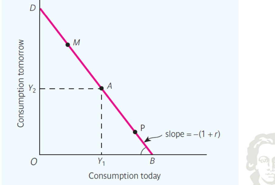
The intertemporal budget line allocates lifetime resources between consumption today and tomorrow. Its slope is minus the gross interest factor, −(1+r): giving up one unit today finances 1+r units tomorrow.
An indifference curve: utility held constant
Fit to text
Scroll horizontally to inspect the labels and values.
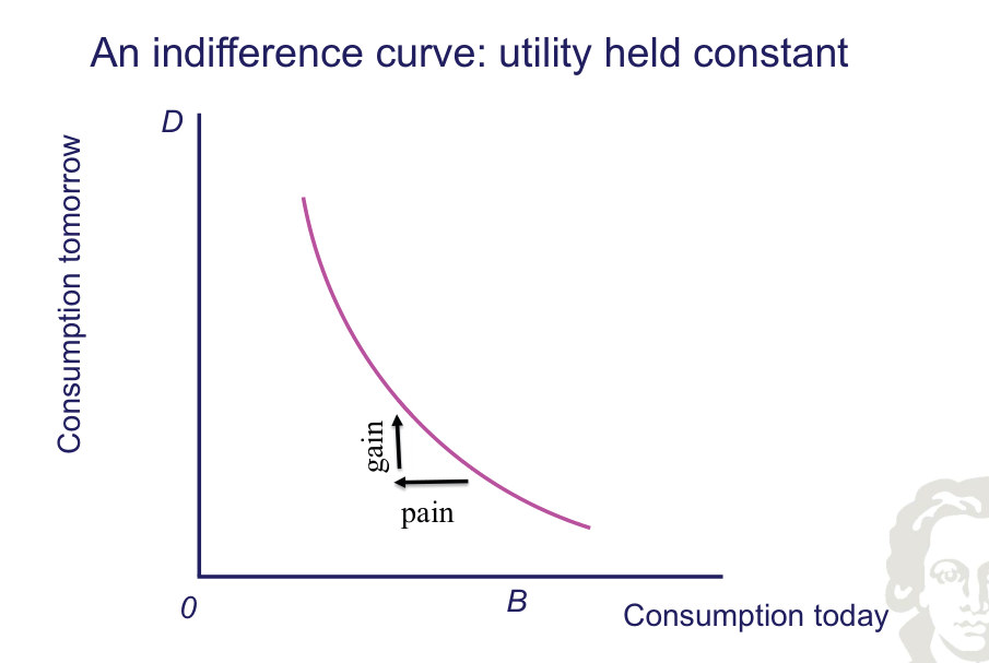
An intertemporal indifference curve joins consumption bundles yielding the same utility. Its downward slope represents willingness to substitute future consumption for current consumption; curvature reflects diminishing marginal utility.
Optimal consumption
Fit to text
Scroll horizontally to inspect the labels and values.
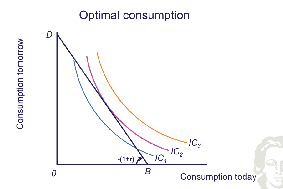
The optimal intertemporal consumption allocation is the tangency between the highest attainable indifference curve and the lifetime budget line. At an interior solution, the intertemporal marginal rate of substitution equals the gross interest factor.
Optimal consumption: borrowing
Fit to text
Scroll horizontally to inspect the labels and values.
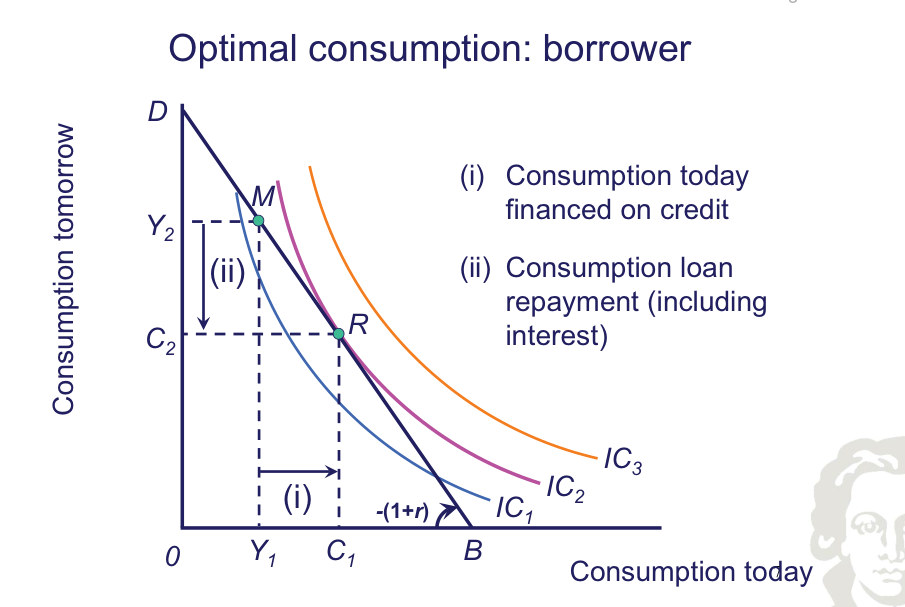
A borrower consumes more than current income and repays principal plus interest from future income. The budget line and preferences determine the optimal amount borrowed.
Optimal consumption: lending
Fit to text
Scroll horizontally to inspect the labels and values.
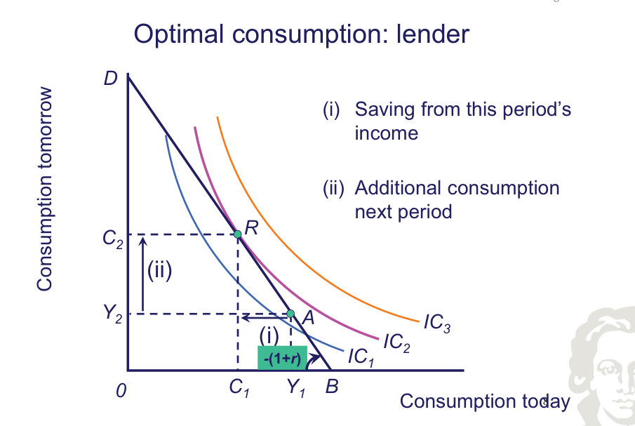
A lender consumes less than current income and carries saving forward with interest. The optimum balances the utility cost of lower current consumption against the utility benefit of higher future consumption.
Tools Of The Trade
The RBC model emphasizes optimizing intertemporal choices, capital accumulation and real productivity shocks. New Keynesian models retain dynamic optimization while adding nominal price-setting frictions, making monetary-policy transmission and stabilization central to the analysis.
Synthesis
Behavioral equations derived from intertemporal optimizing agents can respond to changes in incentives, which is essential for structural policy analysis.
3. Measuring business cycles: empirical regularities
Introduction
Before asking whether a model explains recessions and expansions, we must decide what counts as a cyclical deviation in the data. Raw output levels mix long-run growth with shorter-run fluctuations. Trend extraction is therefore a substantive modelling and measurement choice, not a cosmetic correction.
The empirical analysis uses linear trends, Hodrick–Prescott filtering and band-pass/high-pass ideas, and shows the transformation of consumption, investment, government expenditure and international flows across different economies. A model should be evaluated using compatible definitions, frequencies, seasonal adjustments and filtering rules.
Two sets of moments matter. Kaldor's facts characterize balanced growth over long horizons: labor productivity and capital per worker tend to grow, while the return to capital, the capital–output ratio and factor income shares are comparatively stable. Business-cycle moments characterize volatility, comovement and timing: investment is typically far more volatile than output, while consumption fluctuates less and several aggregates move procyclically.
Integrated theoretical explanation
Observed macroeconomic series combine several time scales. Long-run growth reflects changes in technology, labor and capital; the medium-run component contains recurring expansions and contractions; and very short-run variation can be seasonal or irregular. These are analytic distinctions, not three separately observable objects. An increase in real GDP from one quarter to the next may occur even when output is below its estimated trend, because positive growth and a negative output gap are different statements. Measuring the business cycle therefore requires an explicit choice about the underlying series and the meaning of its trend.
The contrast between nominal output and real output is fundamental. A nominal expenditure series can increase because of higher prices, greater quantities or both; a real series aims to remove the price-level component. Per-capita or per-worker measures answer still different questions, because they adjust for changes in population or labor input. Taking logarithms can make trends more comparable across time and allows log deviations to be interpreted approximately as proportional departures. Before computing a standard deviation or correlation, the sample period, deflator, treatment of seasonality, transformation and measurement units should all be consistent across series.
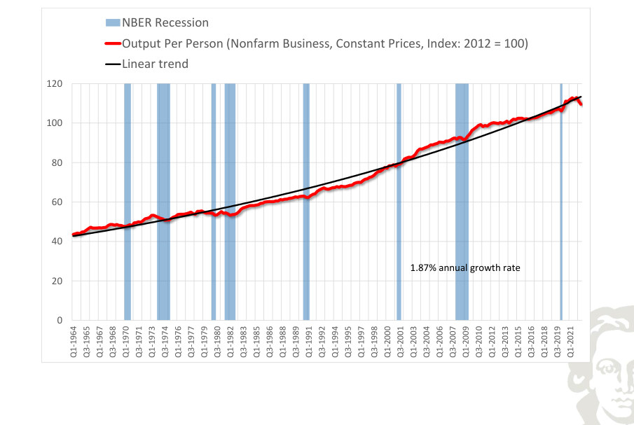
A deterministic linear trend in log output describes a constant average proportional growth rate. Subtracting it yields an output cycle measured relative to this preselected path. Its simplicity is an advantage, but the method is potentially misleading if trend growth changes over time. Conversely, allowing the trend to move too easily can remove genuine cyclical variation. A mechanical trend estimate is consequently not a neutral fact about the data: it embodies a view about which movements are persistent enough to count as growth rather than business cycles.
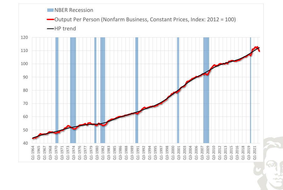
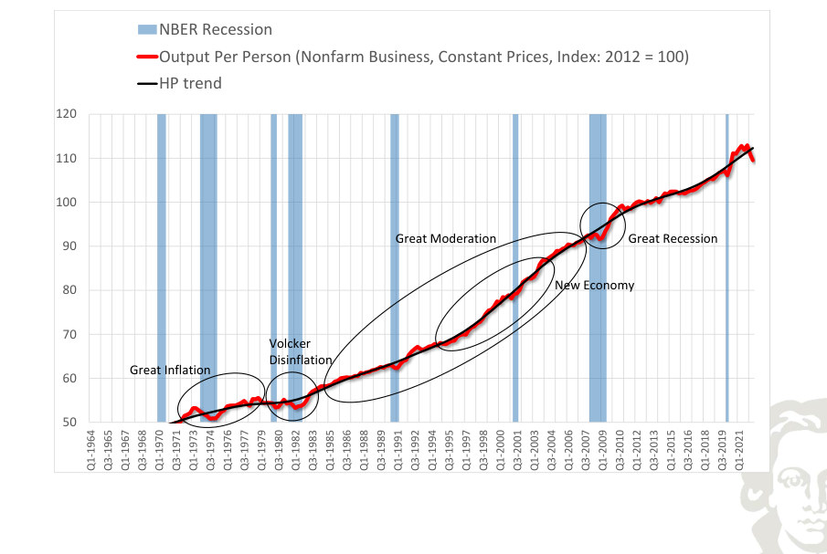
The Hodrick–Prescott filter chooses a smooth trend by minimizing the sum of squared deviations from the observations plus a penalty on variation in the trend's slope. A higher smoothing parameter makes the estimated trend less flexible. The cycle is the difference between the original series and this trend. The procedure is convenient because it produces an operational definition without specifying a full structural model, but it is sensitive to the smoothing choice and to the sample end points. Since the current end of a time series has no future observations available to anchor its trend, revisions can be especially large there.
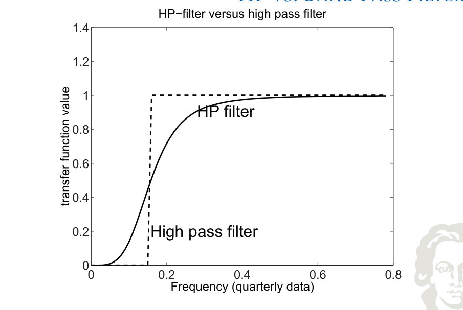
Band-pass filters address frequency ranges more explicitly. Rather than isolating all residual variation after a smooth trend is removed, a band-pass approach attempts to retain fluctuations with durations within a prescribed interval. This emphasizes that the business cycle is partly defined by periodicity. Filters need not give identical turning points or amplitudes, even when applied to the same national-accounts data. Empirical model comparisons are strongest when the simulated and observed series are subjected to the same transformation instead of comparing unfiltered model deviations with filtered data.
The long-run stylized facts associated with Nicholas Kaldor describe the broad shape of economic growth. Output per worker and capital per worker tend to rise over time, while the capital–output ratio, the rate of return on capital and labor and capital income shares are comparatively stable in a balanced-growth characterization. The Solow model with suitable production technology can reconcile these facts: labor-augmenting technical progress raises productivity, while capital deepening keeps the ratio of capital to effective labor near its stationary value. These properties concern a long-horizon trend and should not be confused with the amplitude of quarterly cyclical fluctuations.
Business-cycle moments instead describe how variables move around their trends. Standard deviation measures typical cyclical dispersion; relative standard deviation divides this measure by that of output. A positive contemporaneous correlation with output indicates procyclical comovement, while a negative one indicates countercyclical movement. Lead–lag correlations examine the timing of a variable's fluctuations relative to output. The broad empirical pattern motivating the RBC benchmark is that consumption is relatively smooth, investment is considerably more volatile than output, and hours worked and many private spending aggregates are procyclical. Capital stock itself usually adjusts much more gradually than gross investment.
The country and component comparisons matter because no single historical plot can establish a universal regularity. A recession can be global or concentrated in one economy; import and export series reflect external demand and national-accounting differences; and public expenditure need not follow the same cyclical pattern as private investment. When looking at output, consumption, investment, public demand or external flows across different geographic samples, the purpose is to determine which properties are sufficiently persistent to serve as meaningful quantitative targets. The RBC model should be judged on a defined collection of moments, not on whether one chart happens to look similar.
Formal framework and essential relationships
Three concepts of cyclical data
On the log scale, a deviation can be read approximately as a percentage above or below trend. Trends and cycles are measured constructs, not directly observed separate quantities.
The Hodrick–Prescott filter selects the trend τ to trade off fidelity to the observed series against smoothness of its growth. The parameter λ penalizes changes in the trend slope.
Kaldor facts and cyclical moments must not be confused
| Object | Long-run / business-cycle role | Relevant measure |
|---|---|---|
| Output per worker | Growth regularity | Y/L |
| Capital intensity | Growth regularity | K/L |
| Factor income shares | Growth regularity | wL/Y and rK/Y |
| Relative volatility | Business-cycle dispersion | sd(xᶜ)/sd(Yᶜ) |
| Contemporaneous correlation | Business-cycle comovement | corr(xᶜ,Yᶜ) |
| Lead–lag correlation | Timing | corr(xₜ₊ⱼᶜ,Yₜᶜ) |
Empirical business-cycle moments
| Series | Standard deviation | Relative to GDP |
|---|---|---|
| GDP | 0.016 | 1.0 |
| Non-durable consumption | 0.014 | 0.906 |
| Investment | 0.064 | 4.134 |
| Capital | 0.007 | 0.446 |
| Total hours | 0.02 | 1.315 |
| Employment | 0.014 | 0.879 |
| Average hours | 0.009 | 0.592 |
| Labor productivity | 0.01 | 0.644 |
| TFP | 0.012 | 0.774 |
These empirical moments refer to the defined series and detrending transformations. The quantitative model should be evaluated using moments computed on the same basis.
Explanations, derivations and empirical applications
What Are Business Cycles?
Business-cycle statistics summarize recurring comovement and variability in macroeconomic data. Results depend on how the raw series are transformed and which frequency range is taken to represent the cycle.
Business cycles are broad fluctuations in aggregate economic activity rather than movements in a single sector. The classic characterization of Burns and Mitchell distinguishes expansions spread across many activities from similarly widespread contractions, revivals and subsequent expansions. Their duration is not fixed: historical cycles have varied considerably in length. Their defining characteristics include comovement, persistence and a recognizable sequence of phases.
Why The Cycle?
Studying aggregate fluctuations requires tracking many interrelated variables rather than treating output alone as the cycle. Consumption, investment, labor inputs, productivity and other indicators can have different amplitudes and timing. In the spirit of Sims’s argument for confronting macroeconomic theory with reality, statistical models and carefully transformed observations supply a common arena in which competing mechanisms can be quantitatively evaluated.
Decomposing observed macroeconomic data
A common decomposition expresses an observed economic series as a trend component plus a cyclical deviation. The appropriate trend may be suggested by theory, as in the balanced growth path of the neoclassical growth model, but not every variable has a constant trend after simple normalization. Hours per worker, participation and population-related measures may exhibit their own long-run movements. Therefore, the chosen decomposition must be justified separately for the variables being studied.
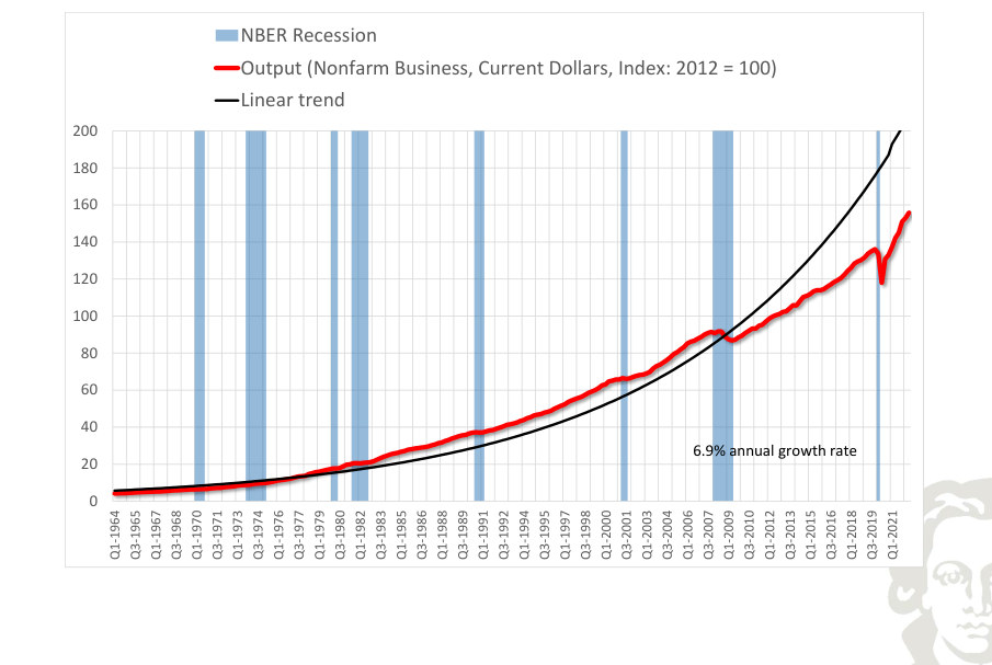
NBER Recession Output (Nonfarm Business, Current Dollars, Index: 2012 = 100)
Fit to text
Scroll horizontally to inspect the labels and values.
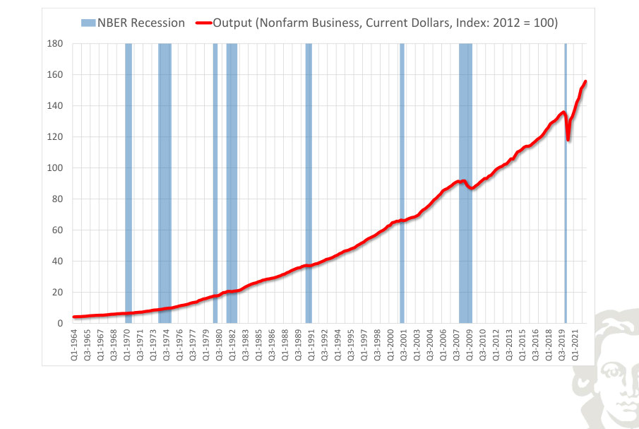
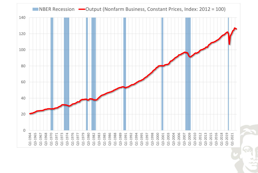
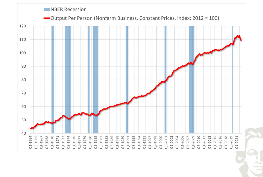
Separating a stochastic cycle from an estimated trend requires selecting an observed series, a trend specification and a smoothing convention. Changes in the trend estimator alter the measured cycle; recession bands provide historical context rather than mechanically defining the cyclical component.
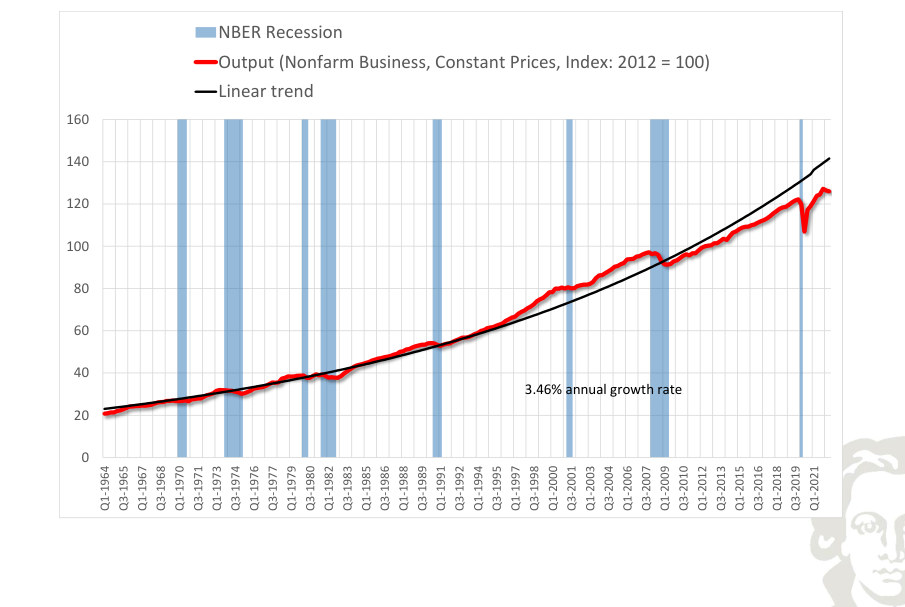
Linear Trend (In Logs)
A linear trend in log output imposes a constant average growth rate. The cyclical component is the difference between observed log output and its estimated trend:
Using real rather than nominal output removes price-level changes, but a fixed trend can still miss changes in growth. Statistical filters allow a time-varying trend.
NBER Recession
Fit to text
Scroll horizontally to inspect the labels and values.
NBER Recession Output (Nonfarm Business, Constant Prices, Index: 2012 = 100)
Fit to text
Scroll horizontally to inspect the labels and values.
NBER Recession
Fit to text
Scroll horizontally to inspect the labels and values.
NBER Recession Deviations from trend
Fit to text
Scroll horizontally to inspect the labels and values.
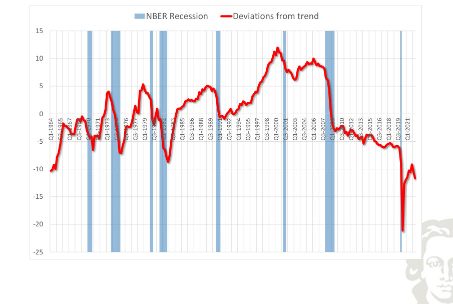
Detrended macroeconomic activity for the selected economy highlights movements above and below the estimated long-run path. The horizontal zero line is a normalization relative to the chosen filter, not a literal condition of zero production. Compare the timing and amplitude of these fluctuations with the corresponding output series.
NBER Recession
Fit to text
Scroll horizontally to inspect the labels and values.
Fit to text
Scroll horizontally to inspect the labels and values.
A Statistical Method: Hodrick-Prescott Filter
Separate the observed series into trend and cycle. The HP filter chooses the trend to minimize:
A larger λ penalizes changes in trend growth more heavily. At λ = 0 the trend follows the data exactly; as λ grows without bound, the fitted trend approaches a straight line.
NBER Recession
Fit to text
Scroll horizontally to inspect the labels and values.
Fit to text
Scroll horizontally to inspect the labels and values.
Fit to text
Scroll horizontally to inspect the labels and values.
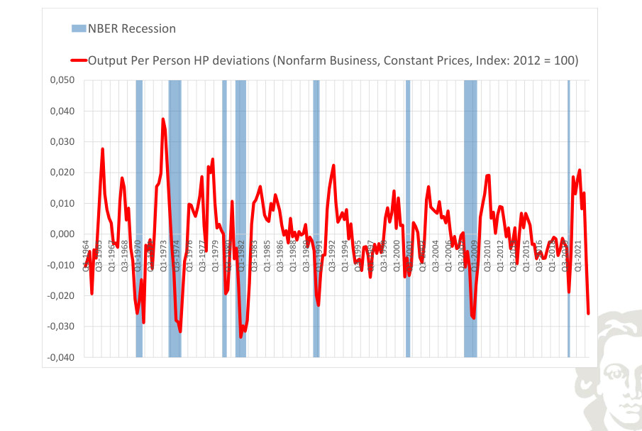
Fit to text
Scroll horizontally to inspect the labels and values.
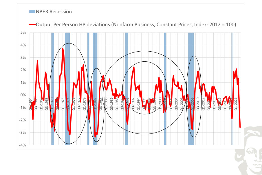
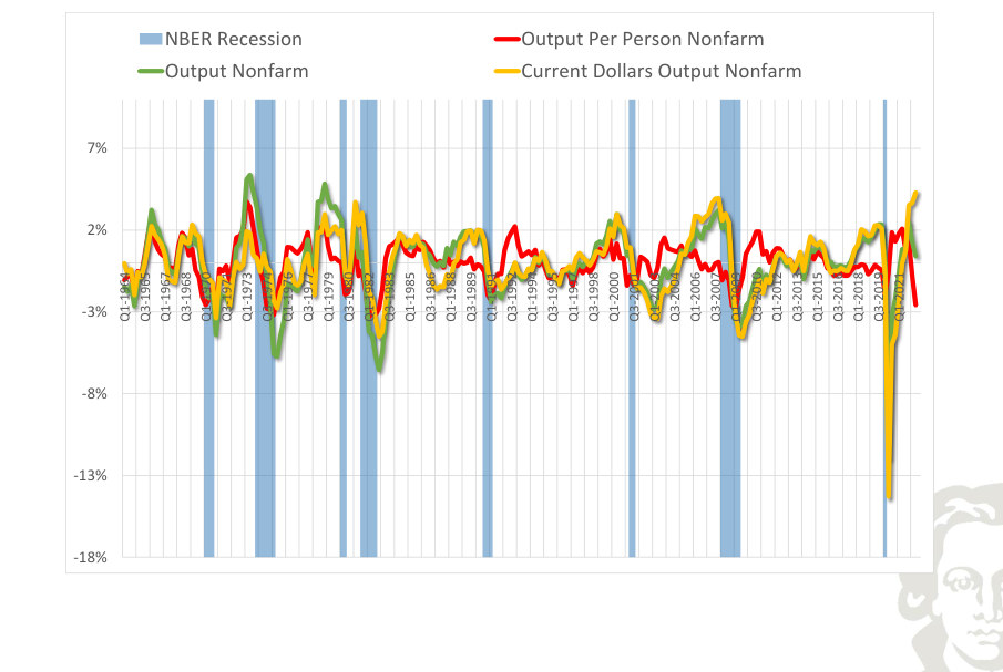
NBER Recession Output Per Person Nonfarm
Fit to text
Scroll horizontally to inspect the labels and values.
HP Vs. Band Pass Filter
Fit to text
Scroll horizontally to inspect the labels and values.
Stylized Macro Facts
National expenditure and its transformations:
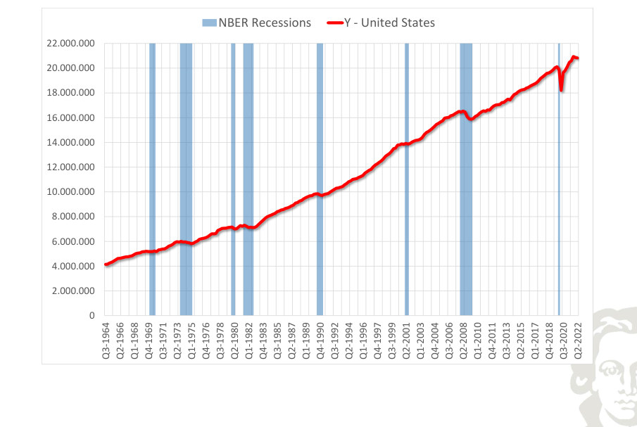
The growth formula compares consecutive observations. The time interval and any annualization must be specified. Source for the country series: OECD.
USA · country series
NBER Recessions Y - United States
Fit to text
Scroll horizontally to inspect the labels and values.
NBER Recessions Y - United States (Annual Growth)
Fit to text
Scroll horizontally to inspect the labels and values.
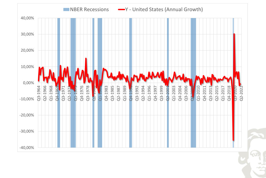
The plotted growth rate of real output for the United States measures the change in activity under the frequency and rate convention of the series. Negative growth and below-trend growth are different concepts; comparing them helps identify contractions without assuming that every slowing constitutes a recession.
NBER Recessions Y - United States (Annual Trend Growth)
Fit to text
Scroll horizontally to inspect the labels and values.
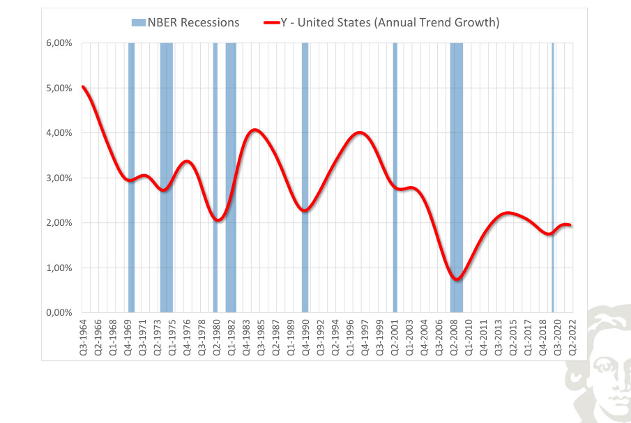
The smoothed growth path of real output in the United States describes the slower-moving change in the rate of expansion. It should not be equated with the cyclical component: the trend-growth series may slow even when the level of activity continues to rise.
NBER Recessions Y - United States (Deviations from Trend)
Fit to text
Scroll horizontally to inspect the labels and values.
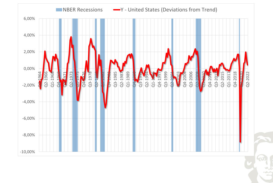
Detrended real output for the United States highlights movements above and below the estimated long-run path. The horizontal zero line is a normalization relative to the chosen filter, not a literal condition of zero production. Compare the timing and amplitude of these fluctuations with the corresponding output series.
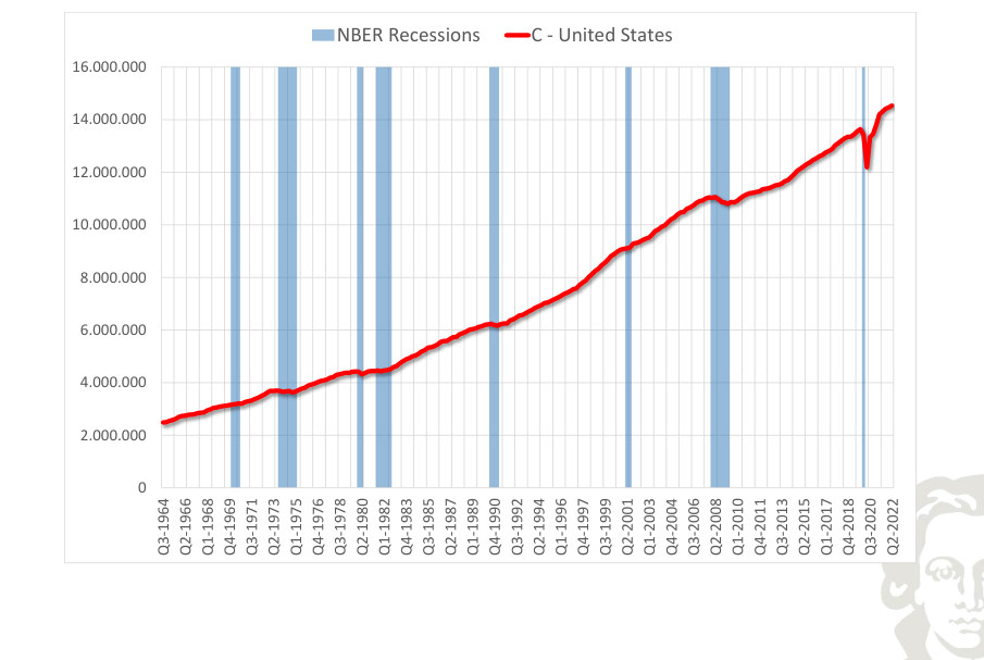
NBER Recessions C - United States
Fit to text
Scroll horizontally to inspect the labels and values.
NBER Recessions C - United States (Annual Growth)
Fit to text
Scroll horizontally to inspect the labels and values.
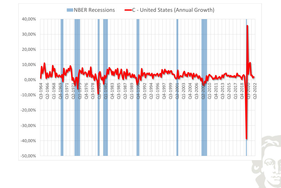
The plotted growth rate of consumption for the United States measures the change in activity under the frequency and rate convention of the series. Negative growth and below-trend growth are different concepts; comparing them helps identify contractions without assuming that every slowing constitutes a recession.
NBER Recessions C - United States (Annual Trend Growth)
Fit to text
Scroll horizontally to inspect the labels and values.
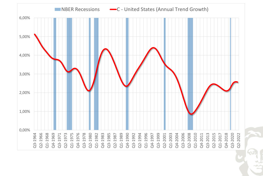
The smoothed growth path of consumption in the United States describes the slower-moving change in the rate of expansion. It should not be equated with the cyclical component: the trend-growth series may slow even when the level of activity continues to rise.
NBER Recessions C - United States (Deviations from Trend)
Fit to text
Scroll horizontally to inspect the labels and values.
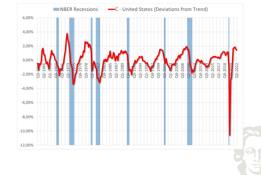
Detrended consumption for the United States highlights movements above and below the estimated long-run path. The horizontal zero line is a normalization relative to the chosen filter, not a literal condition of zero production. Compare the timing and amplitude of these fluctuations with the corresponding output series.
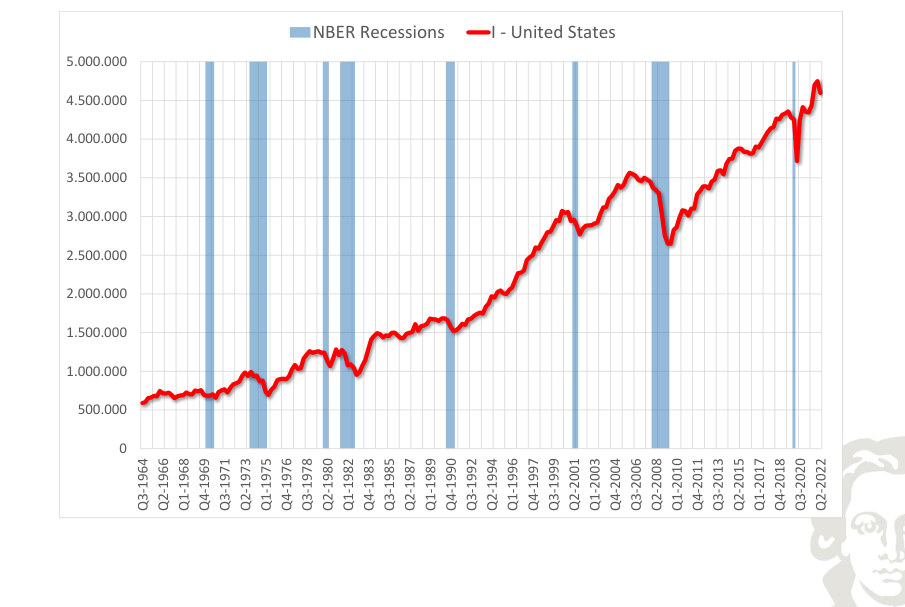
NBER Recessions I - United States
Fit to text
Scroll horizontally to inspect the labels and values.
NBER Recessions I - United States (Annual Growth)
Fit to text
Scroll horizontally to inspect the labels and values.
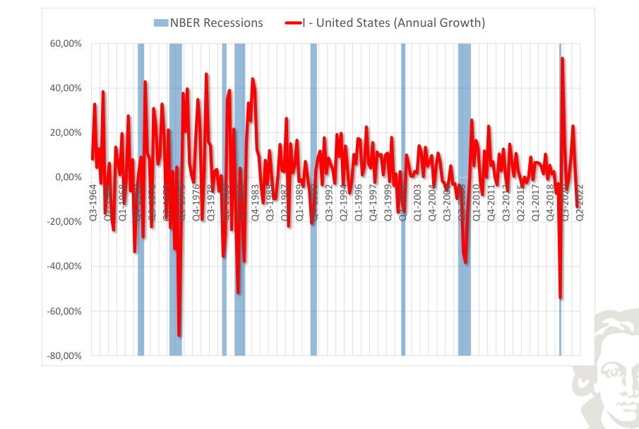
The plotted growth rate of investment for the United States measures the change in activity under the frequency and rate convention of the series. Negative growth and below-trend growth are different concepts; comparing them helps identify contractions without assuming that every slowing constitutes a recession.
NBER Recessions I - United States (Annual Trend Growth)
Fit to text
Scroll horizontally to inspect the labels and values.
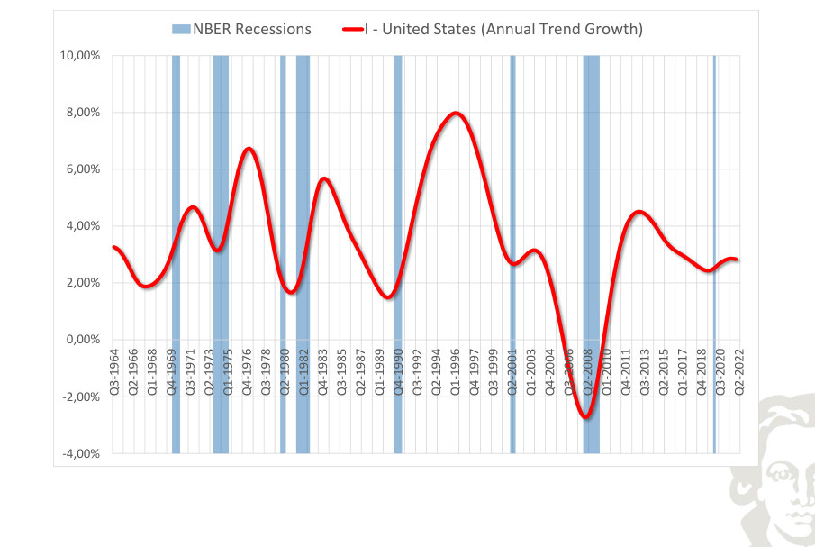
The smoothed growth path of investment in the United States describes the slower-moving change in the rate of expansion. It should not be equated with the cyclical component: the trend-growth series may slow even when the level of activity continues to rise.
NBER Recessions I - United States (Deviations from Trend)
Fit to text
Scroll horizontally to inspect the labels and values.
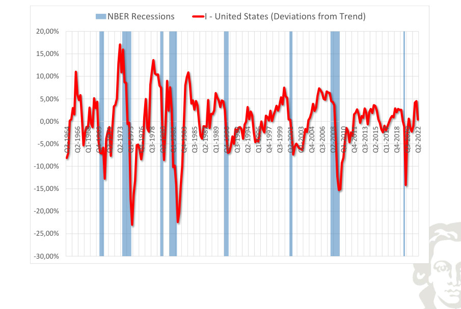
Detrended investment for the United States highlights movements above and below the estimated long-run path. The horizontal zero line is a normalization relative to the chosen filter, not a literal condition of zero production. Compare the timing and amplitude of these fluctuations with the corresponding output series.
NBER Recessions G - United States
Fit to text
Scroll horizontally to inspect the labels and values.
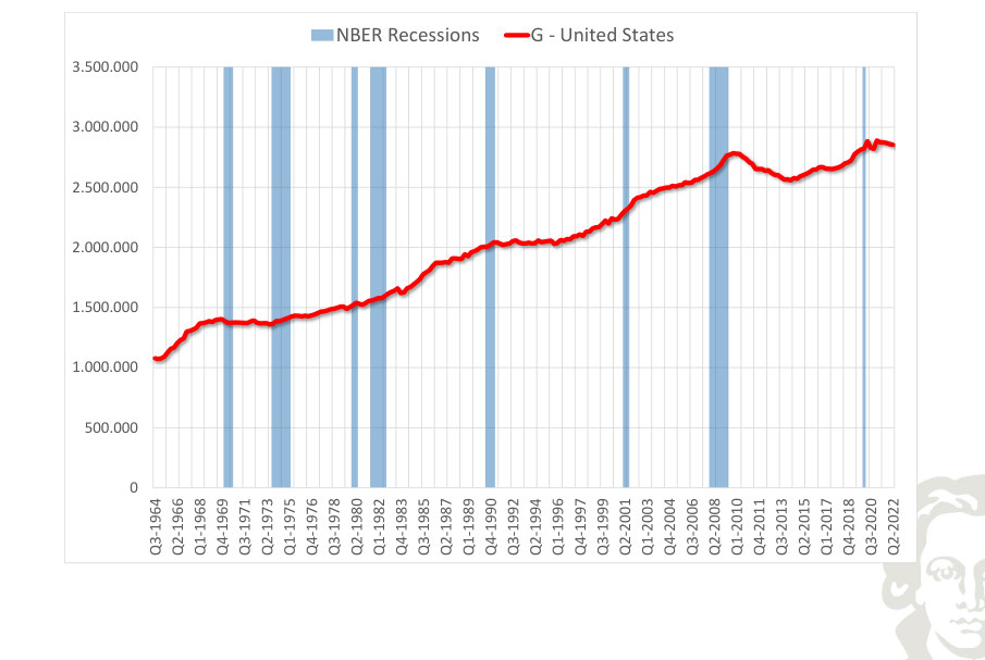
NBER Recessions G - United States (Annual Growth)
Fit to text
Scroll horizontally to inspect the labels and values.
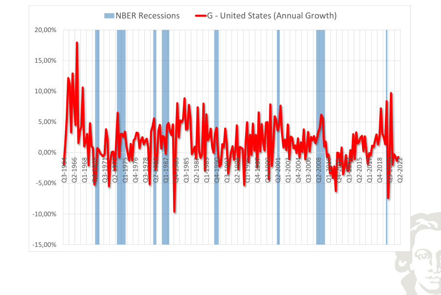
The plotted growth rate of government expenditure for the United States measures the change in activity under the frequency and rate convention of the series. Negative growth and below-trend growth are different concepts; comparing them helps identify contractions without assuming that every slowing constitutes a recession.
NBER Recessions G - United States (Annual Trend Growth)
Fit to text
Scroll horizontally to inspect the labels and values.
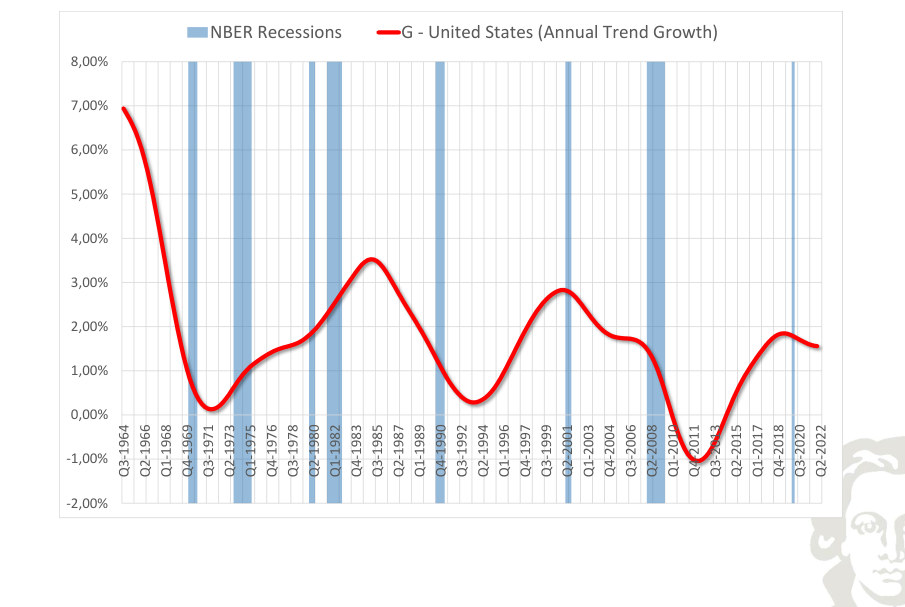
The smoothed growth path of government expenditure in the United States describes the slower-moving change in the rate of expansion. It should not be equated with the cyclical component: the trend-growth series may slow even when the level of activity continues to rise.
NBER Recessions G - United States (Deviations from Trend)
Fit to text
Scroll horizontally to inspect the labels and values.
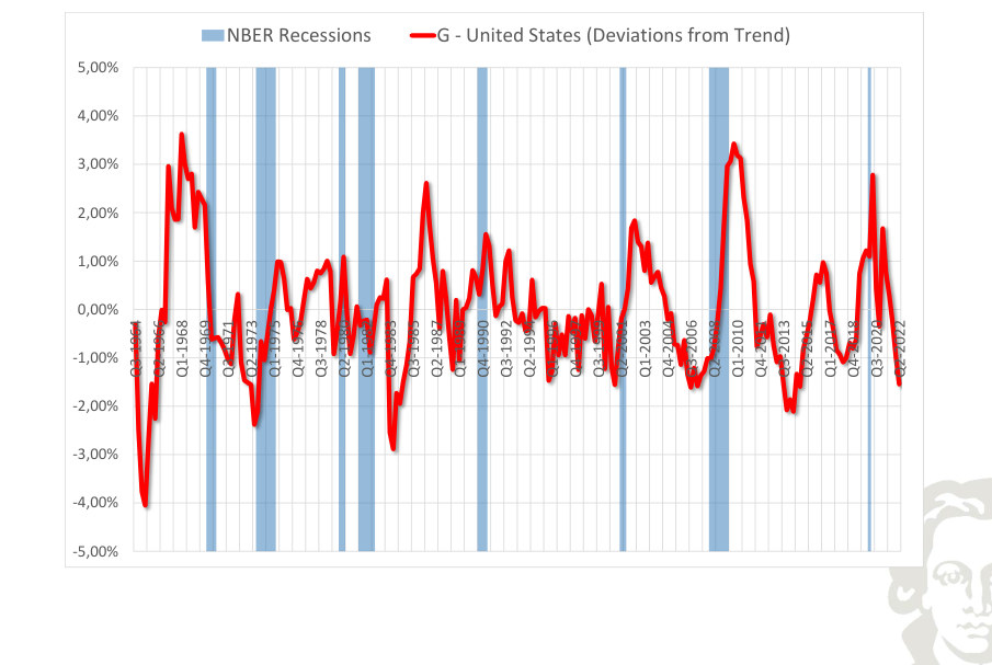
Detrended government expenditure for the United States highlights movements above and below the estimated long-run path. The horizontal zero line is a normalization relative to the chosen filter, not a literal condition of zero production. Compare the timing and amplitude of these fluctuations with the corresponding output series.
NBER Recessions X - United States
Fit to text
Scroll horizontally to inspect the labels and values.
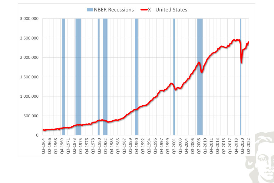
NBER Recessions X - United States (Annual Growth)
Fit to text
Scroll horizontally to inspect the labels and values.
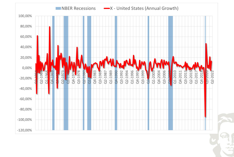
The plotted growth rate of exports for the United States measures the change in activity under the frequency and rate convention of the series. Negative growth and below-trend growth are different concepts; comparing them helps identify contractions without assuming that every slowing constitutes a recession.
NBER Recessions X - United States (Annual Trend Growth)
Fit to text
Scroll horizontally to inspect the labels and values.
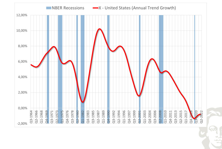
The smoothed growth path of exports in the United States describes the slower-moving change in the rate of expansion. It should not be equated with the cyclical component: the trend-growth series may slow even when the level of activity continues to rise.
NBER Recessions X - United States (Deviations from Trend)
Fit to text
Scroll horizontally to inspect the labels and values.
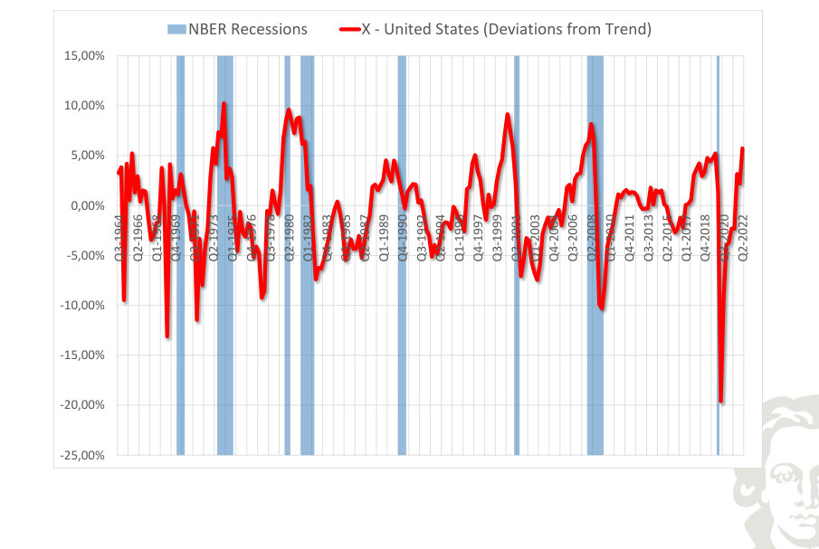
Detrended exports for the United States highlights movements above and below the estimated long-run path. The horizontal zero line is a normalization relative to the chosen filter, not a literal condition of zero production. Compare the timing and amplitude of these fluctuations with the corresponding output series.
NBER Recessions Z - United States
Fit to text
Scroll horizontally to inspect the labels and values.
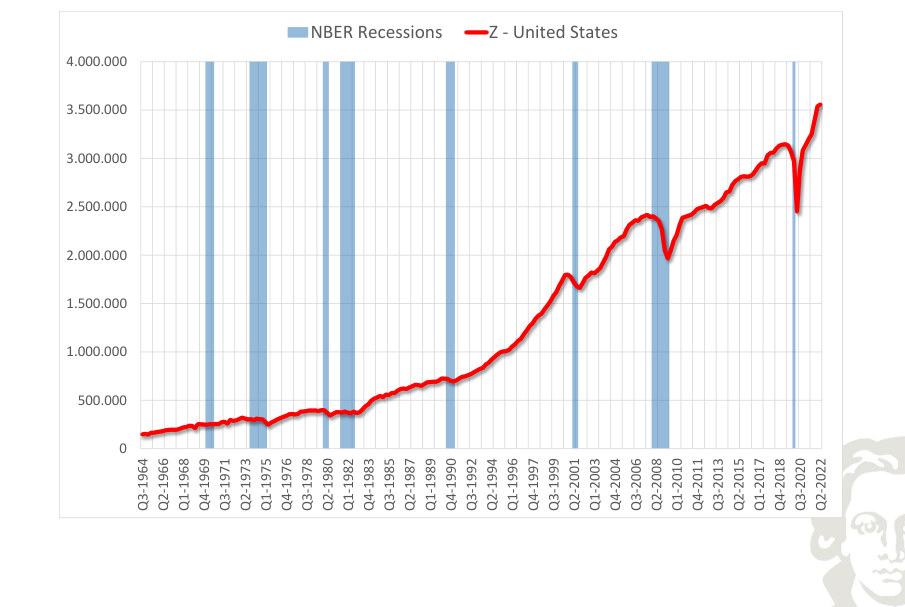
NBER Recessions Z - United States (Annual Growth)
Fit to text
Scroll horizontally to inspect the labels and values.
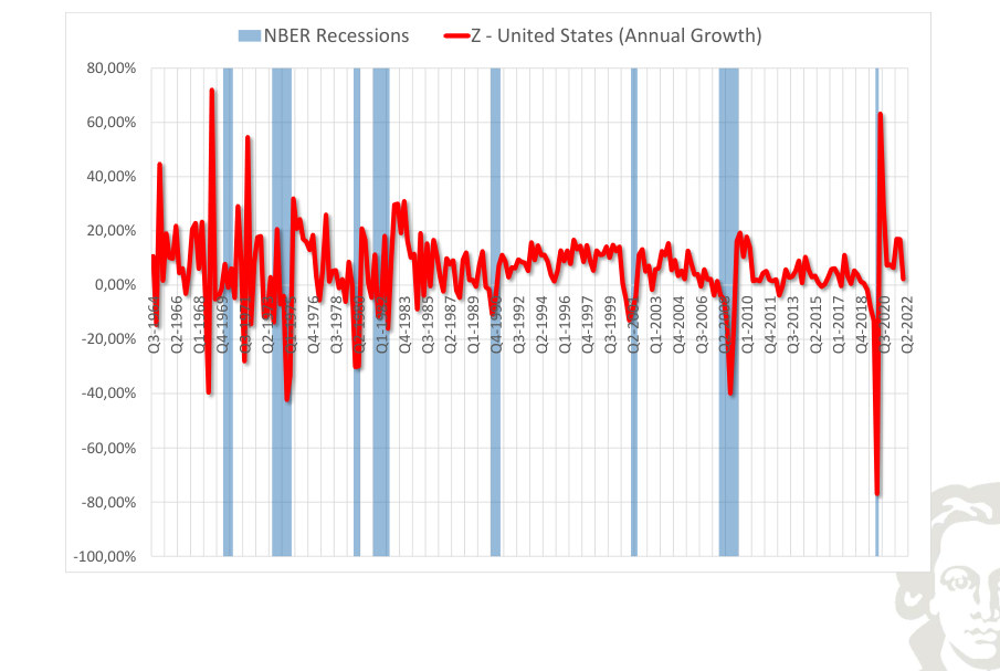
The plotted growth rate of imports for the United States measures the change in activity under the frequency and rate convention of the series. Negative growth and below-trend growth are different concepts; comparing them helps identify contractions without assuming that every slowing constitutes a recession.
NBER Recessions Z - United States (Annual Trend Growth)
Fit to text
Scroll horizontally to inspect the labels and values.
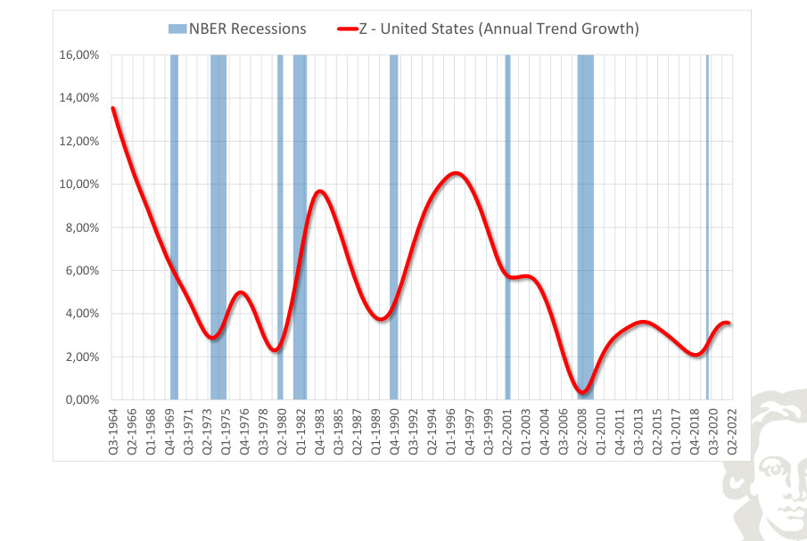
The smoothed growth path of imports in the United States describes the slower-moving change in the rate of expansion. It should not be equated with the cyclical component: the trend-growth series may slow even when the level of activity continues to rise.
NBER Recessions Z - United States (Deviations from Trend)
Fit to text
Scroll horizontally to inspect the labels and values.
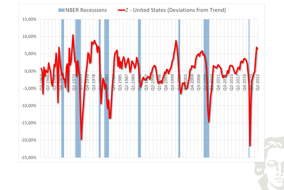
Detrended imports for the United States highlights movements above and below the estimated long-run path. The horizontal zero line is a normalization relative to the chosen filter, not a literal condition of zero production. Compare the timing and amplitude of these fluctuations with the corresponding output series.
EU (18) · country series
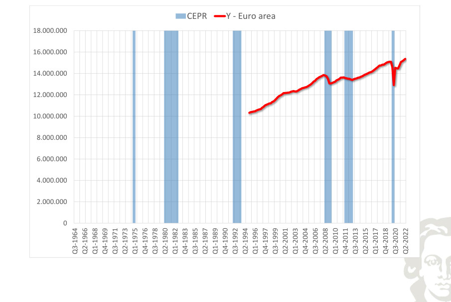
CEPR Y - Euro area
Fit to text
Scroll horizontally to inspect the labels and values.
CEPR Y - Euro area (Annual Growth)
Fit to text
Scroll horizontally to inspect the labels and values.
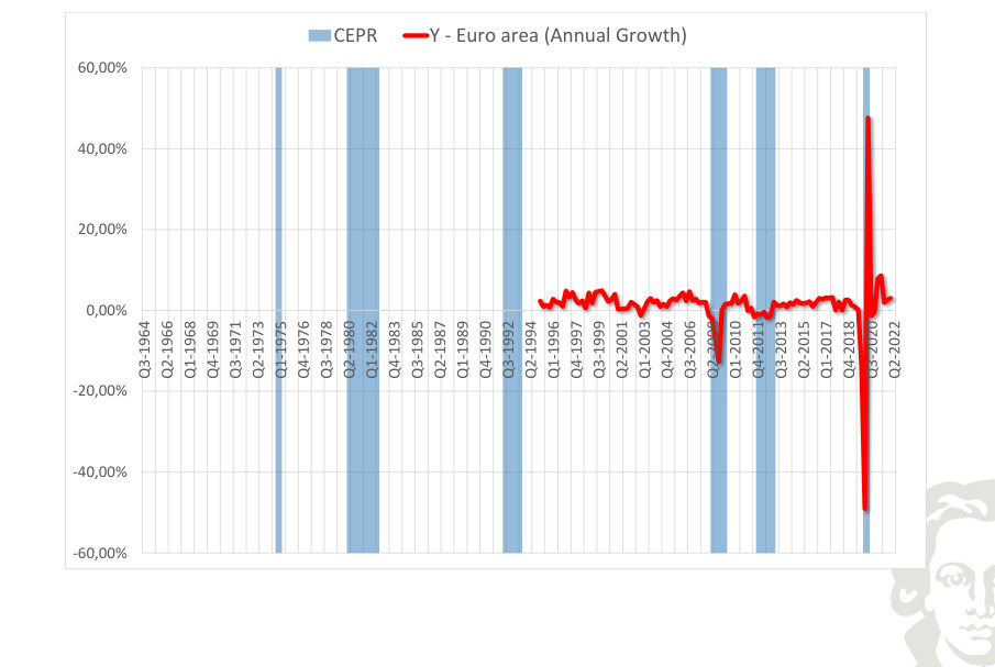
The plotted growth rate of real output for the selected economy measures the change in activity under the frequency and rate convention of the series. Negative growth and below-trend growth are different concepts; comparing them helps identify contractions without assuming that every slowing constitutes a recession.
CEPR Y - Euro area (Annual Trend Growth)
Fit to text
Scroll horizontally to inspect the labels and values.
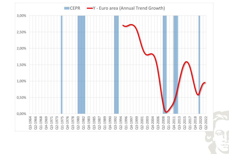
The smoothed growth path of real output in the selected economy describes the slower-moving change in the rate of expansion. It should not be equated with the cyclical component: the trend-growth series may slow even when the level of activity continues to rise.
CEPR Y - Euro area (Deviations from Trend)
Fit to text
Scroll horizontally to inspect the labels and values.
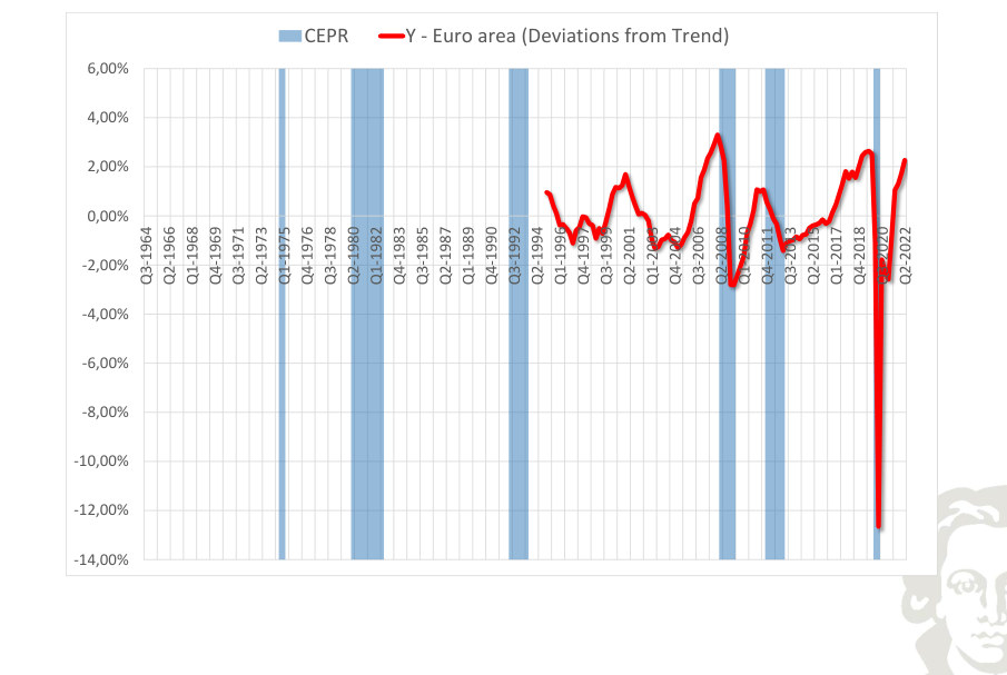
Detrended real output for the selected economy highlights movements above and below the estimated long-run path. The horizontal zero line is a normalization relative to the chosen filter, not a literal condition of zero production. Compare the timing and amplitude of these fluctuations with the corresponding output series.
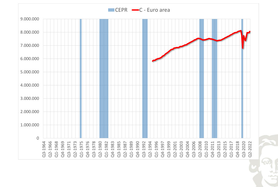
CEPR C - Euro area
Fit to text
Scroll horizontally to inspect the labels and values.
CEPR C - Euro area (Annual Growth)
Fit to text
Scroll horizontally to inspect the labels and values.
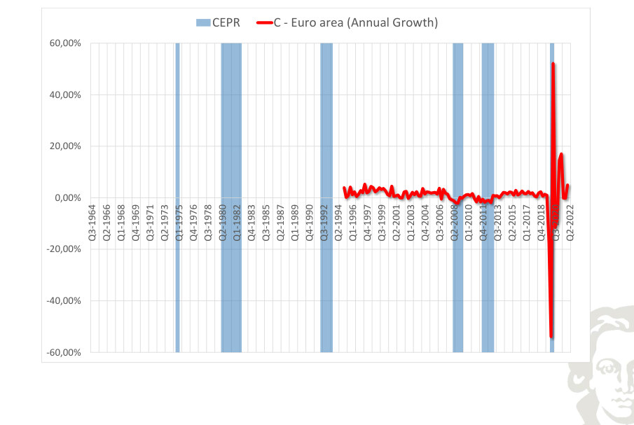
The plotted growth rate of consumption for the selected economy measures the change in activity under the frequency and rate convention of the series. Negative growth and below-trend growth are different concepts; comparing them helps identify contractions without assuming that every slowing constitutes a recession.
CEPR C - Euro area (Annual Trend Growth)
Fit to text
Scroll horizontally to inspect the labels and values.
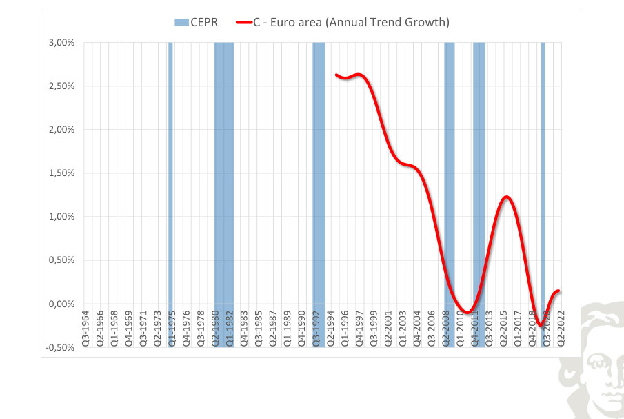
The smoothed growth path of consumption in the selected economy describes the slower-moving change in the rate of expansion. It should not be equated with the cyclical component: the trend-growth series may slow even when the level of activity continues to rise.
CEPR C - Euro Area (Deviations from Trend)
Fit to text
Scroll horizontally to inspect the labels and values.
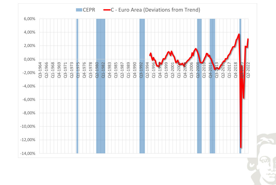
Detrended consumption for the selected economy highlights movements above and below the estimated long-run path. The horizontal zero line is a normalization relative to the chosen filter, not a literal condition of zero production. Compare the timing and amplitude of these fluctuations with the corresponding output series.
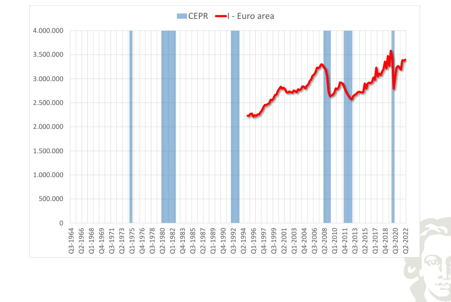
CEPR I - Euro area
Fit to text
Scroll horizontally to inspect the labels and values.
CEPR I - Euro area (Annual Growth)
Fit to text
Scroll horizontally to inspect the labels and values.
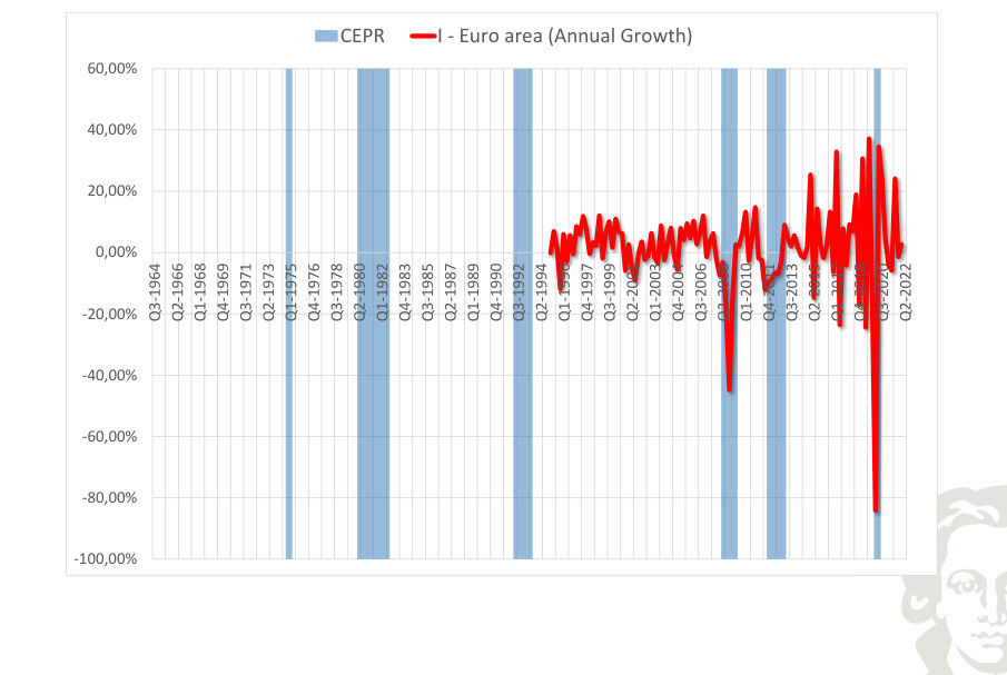
The plotted growth rate of investment for the selected economy measures the change in activity under the frequency and rate convention of the series. Negative growth and below-trend growth are different concepts; comparing them helps identify contractions without assuming that every slowing constitutes a recession.
CEPR I - Euro area (Annual Trend Growth)
Fit to text
Scroll horizontally to inspect the labels and values.
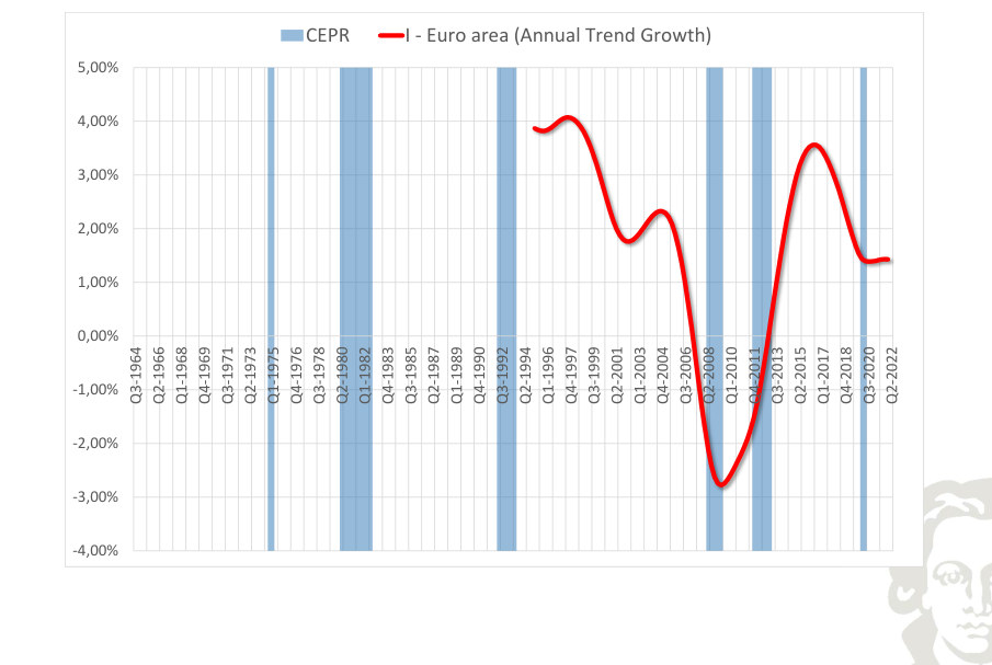
The smoothed growth path of investment in the selected economy describes the slower-moving change in the rate of expansion. It should not be equated with the cyclical component: the trend-growth series may slow even when the level of activity continues to rise.
CEPR I - Euro Area (Deviations from Trend)
Fit to text
Scroll horizontally to inspect the labels and values.
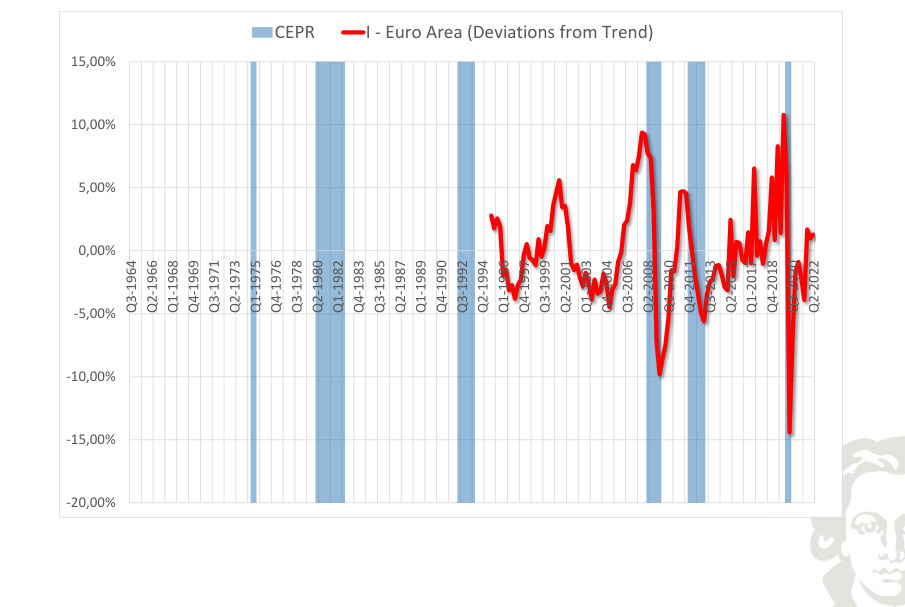
Detrended investment for the selected economy highlights movements above and below the estimated long-run path. The horizontal zero line is a normalization relative to the chosen filter, not a literal condition of zero production. Compare the timing and amplitude of these fluctuations with the corresponding output series.
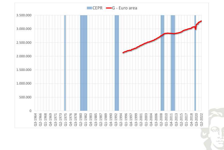
CEPR G - Euro area
Fit to text
Scroll horizontally to inspect the labels and values.
CEPR G - Euro area (Annual Growth)
Fit to text
Scroll horizontally to inspect the labels and values.
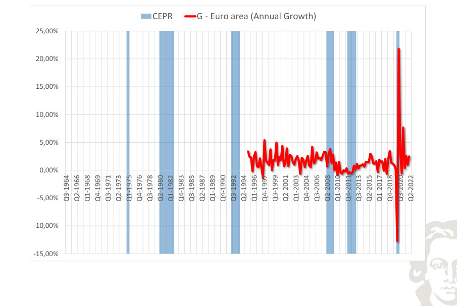
The plotted growth rate of government expenditure for the selected economy measures the change in activity under the frequency and rate convention of the series. Negative growth and below-trend growth are different concepts; comparing them helps identify contractions without assuming that every slowing constitutes a recession.
CEPR G - Euro area (Annual Trend Growth)
Fit to text
Scroll horizontally to inspect the labels and values.
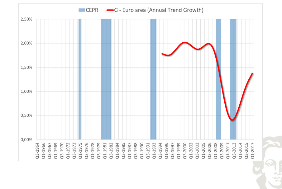
The smoothed growth path of government expenditure in the selected economy describes the slower-moving change in the rate of expansion. It should not be equated with the cyclical component: the trend-growth series may slow even when the level of activity continues to rise.
CEPR G - Euro area (Deviations from Trend)
Fit to text
Scroll horizontally to inspect the labels and values.
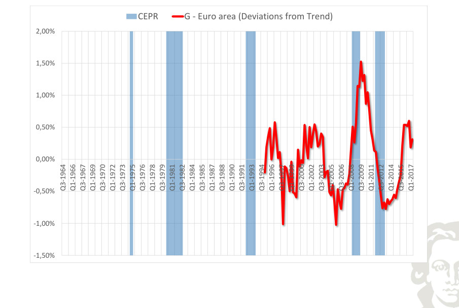
Detrended government expenditure for the selected economy highlights movements above and below the estimated long-run path. The horizontal zero line is a normalization relative to the chosen filter, not a literal condition of zero production. Compare the timing and amplitude of these fluctuations with the corresponding output series.
Japan · country series
OECD Japan Y - Japan
Fit to text
Scroll horizontally to inspect the labels and values.
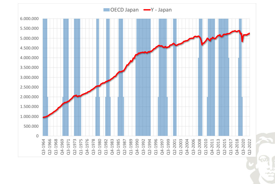
OECD Japan Y - Japan (Annual Growth)
Fit to text
Scroll horizontally to inspect the labels and values.
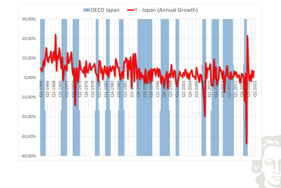
The plotted growth rate of real output for Japan measures the change in activity under the frequency and rate convention of the series. Negative growth and below-trend growth are different concepts; comparing them helps identify contractions without assuming that every slowing constitutes a recession.
OECD Japan Y - Japan (Annual Trend Growth)
Fit to text
Scroll horizontally to inspect the labels and values.
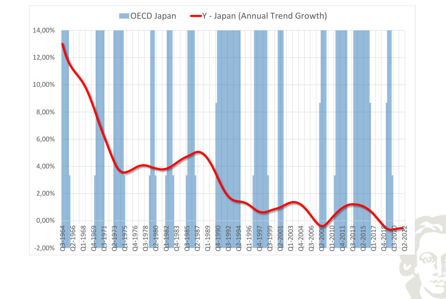
The smoothed growth path of real output in Japan describes the slower-moving change in the rate of expansion. It should not be equated with the cyclical component: the trend-growth series may slow even when the level of activity continues to rise.
OECD Japan Y - Japan (Deviations from Trend)
Fit to text
Scroll horizontally to inspect the labels and values.
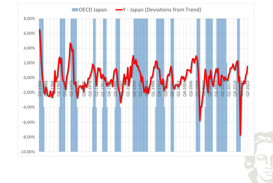
Detrended real output for Japan highlights movements above and below the estimated long-run path. The horizontal zero line is a normalization relative to the chosen filter, not a literal condition of zero production. Compare the timing and amplitude of these fluctuations with the corresponding output series.
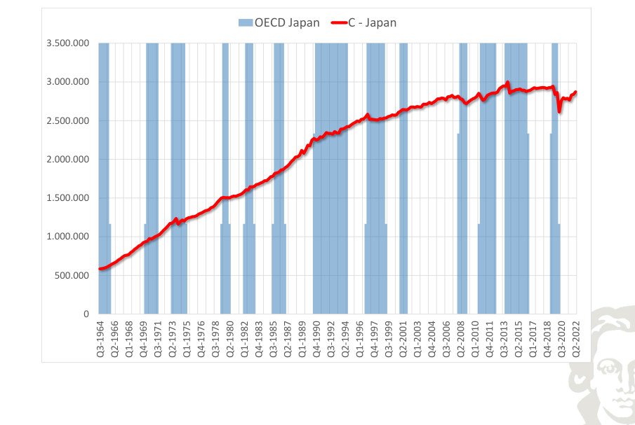
OECD Japan C - Japan
Fit to text
Scroll horizontally to inspect the labels and values.
OECD Japan C - Japan (Annual Growth)
Fit to text
Scroll horizontally to inspect the labels and values.
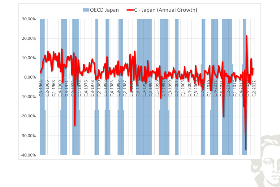
The plotted growth rate of consumption for Japan measures the change in activity under the frequency and rate convention of the series. Negative growth and below-trend growth are different concepts; comparing them helps identify contractions without assuming that every slowing constitutes a recession.
OECD Japan C - Japan (Annual Trend Growth)
Fit to text
Scroll horizontally to inspect the labels and values.
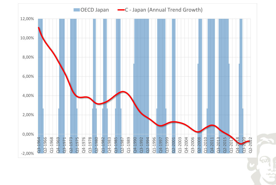
The smoothed growth path of consumption in Japan describes the slower-moving change in the rate of expansion. It should not be equated with the cyclical component: the trend-growth series may slow even when the level of activity continues to rise.
OECD Japan C - Japan (Deviations from Trend)
Fit to text
Scroll horizontally to inspect the labels and values.
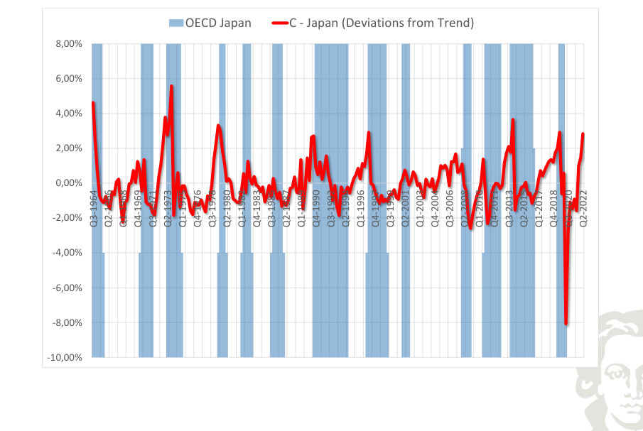
Detrended consumption for Japan highlights movements above and below the estimated long-run path. The horizontal zero line is a normalization relative to the chosen filter, not a literal condition of zero production. Compare the timing and amplitude of these fluctuations with the corresponding output series.
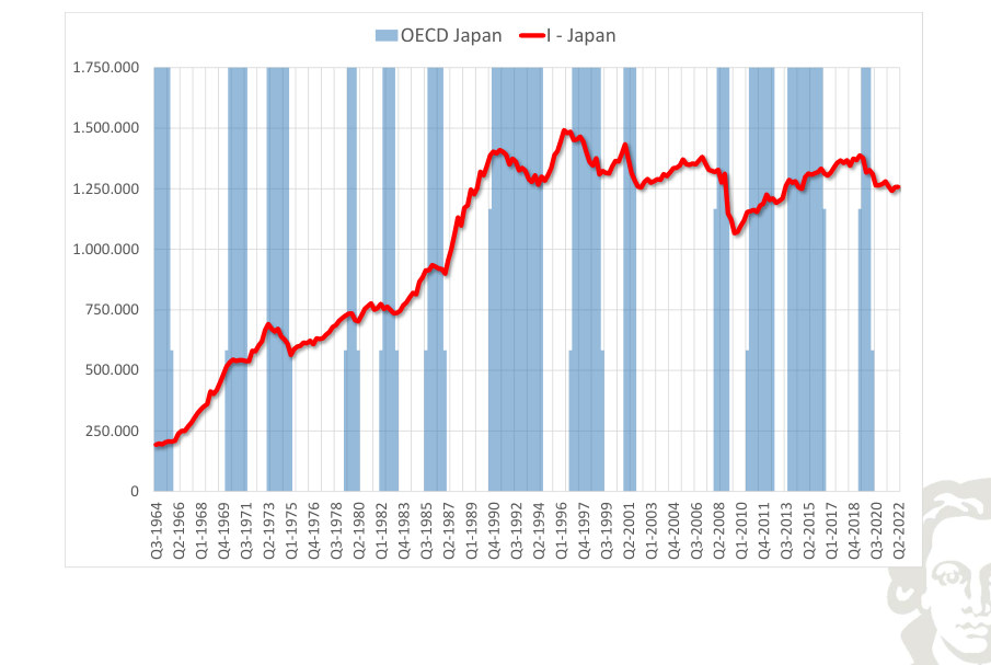
OECD Japan I - Japan
Fit to text
Scroll horizontally to inspect the labels and values.
OECD Japan I - Japan (Annual Growth)
Fit to text
Scroll horizontally to inspect the labels and values.
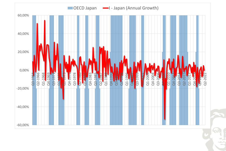
The plotted growth rate of investment for Japan measures the change in activity under the frequency and rate convention of the series. Negative growth and below-trend growth are different concepts; comparing them helps identify contractions without assuming that every slowing constitutes a recession.
OECD Japan I - Japan (Annual Trend Growth)
Fit to text
Scroll horizontally to inspect the labels and values.
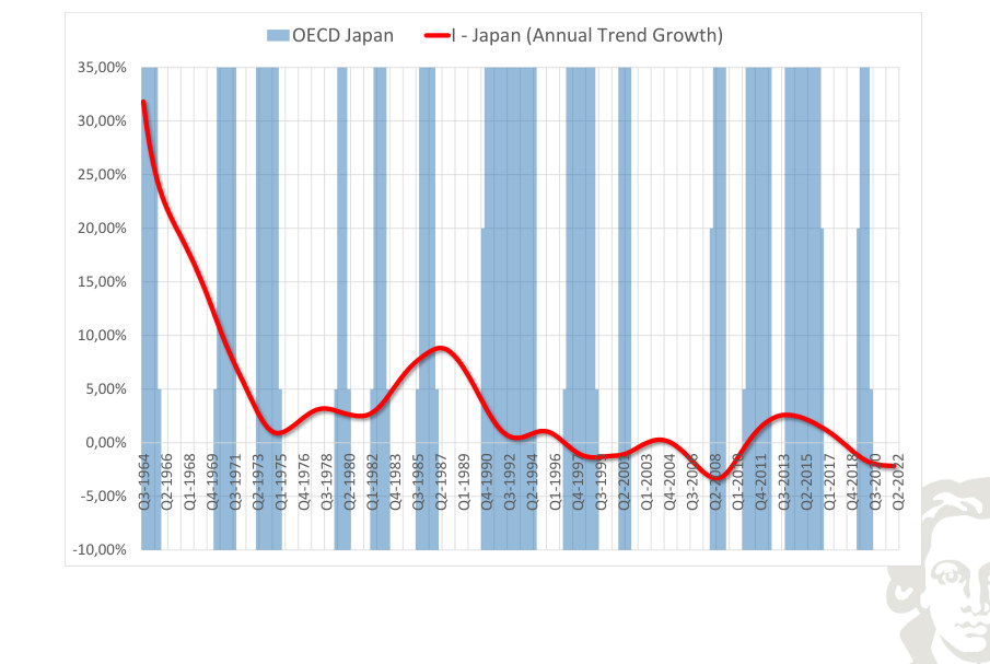
The smoothed growth path of investment in Japan describes the slower-moving change in the rate of expansion. It should not be equated with the cyclical component: the trend-growth series may slow even when the level of activity continues to rise.
OECD Japan I - Japan (Deviations from Trend)
Fit to text
Scroll horizontally to inspect the labels and values.
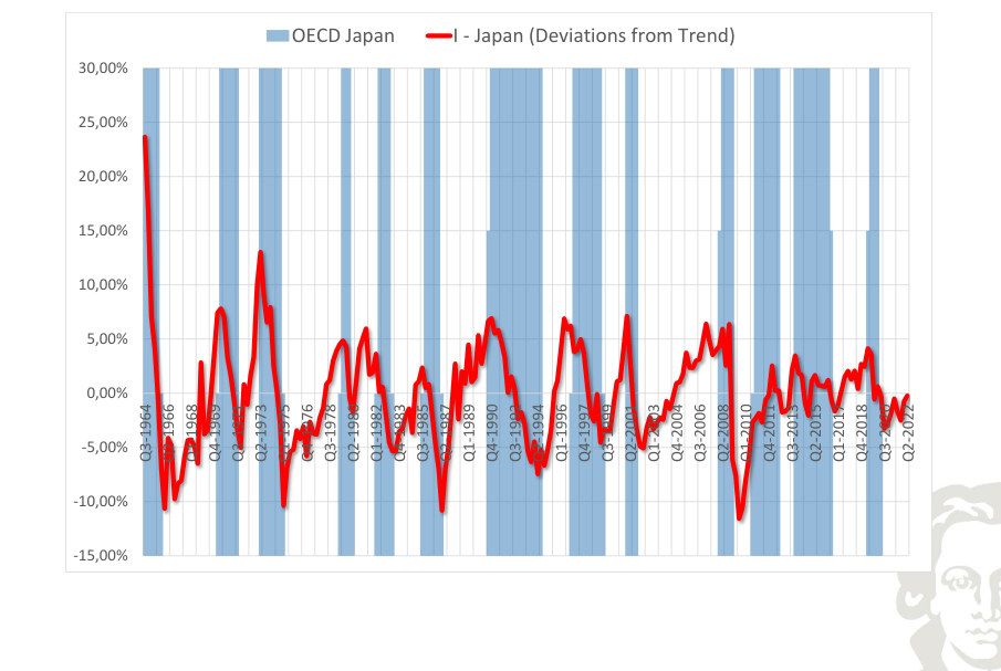
Detrended investment for Japan highlights movements above and below the estimated long-run path. The horizontal zero line is a normalization relative to the chosen filter, not a literal condition of zero production. Compare the timing and amplitude of these fluctuations with the corresponding output series.
OECD Japan G - Japan
Fit to text
Scroll horizontally to inspect the labels and values.
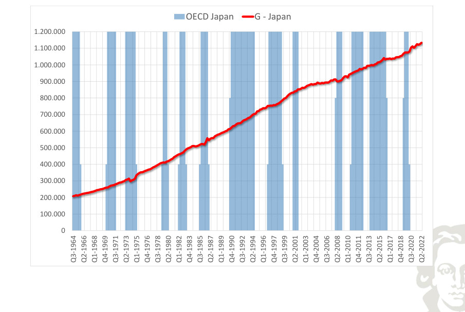
OECD Japan G - Japan (Annual Growth)
Fit to text
Scroll horizontally to inspect the labels and values.
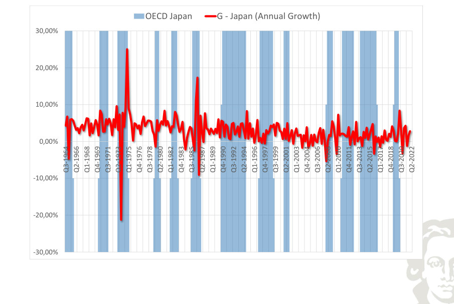
The plotted growth rate of government expenditure for Japan measures the change in activity under the frequency and rate convention of the series. Negative growth and below-trend growth are different concepts; comparing them helps identify contractions without assuming that every slowing constitutes a recession.
OECD Japan G - Japan (Annual Trend Growth)
Fit to text
Scroll horizontally to inspect the labels and values.
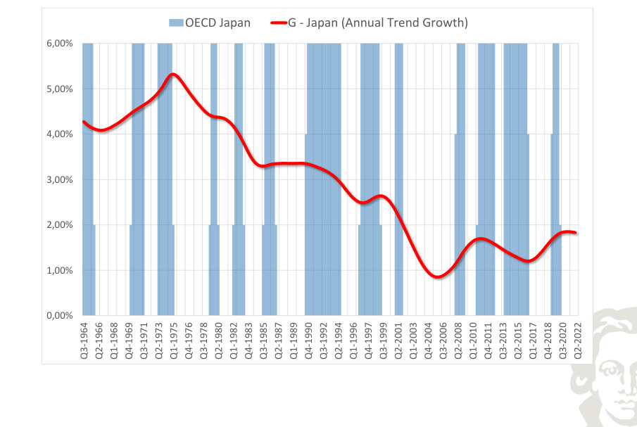
The smoothed growth path of government expenditure in Japan describes the slower-moving change in the rate of expansion. It should not be equated with the cyclical component: the trend-growth series may slow even when the level of activity continues to rise.
OECD Japan G - Japan (Deviations from Trend)
Fit to text
Scroll horizontally to inspect the labels and values.
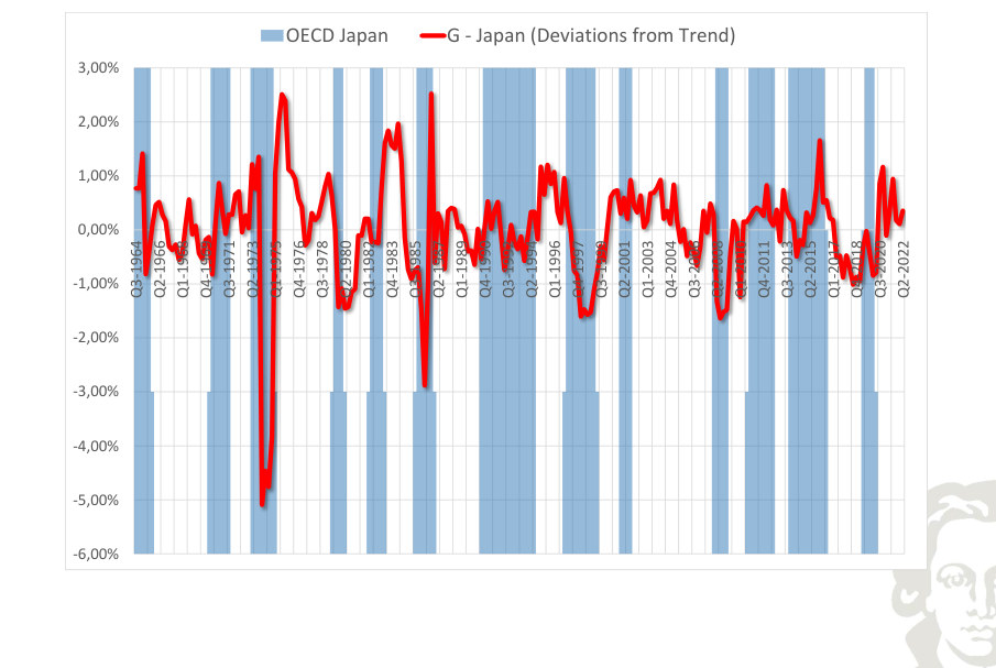
Detrended government expenditure for Japan highlights movements above and below the estimated long-run path. The horizontal zero line is a normalization relative to the chosen filter, not a literal condition of zero production. Compare the timing and amplitude of these fluctuations with the corresponding output series.
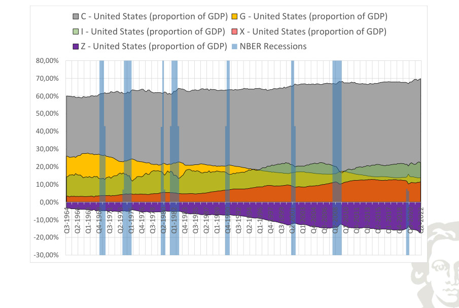
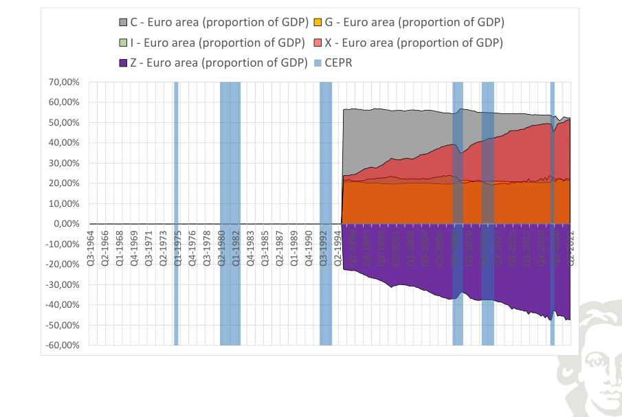
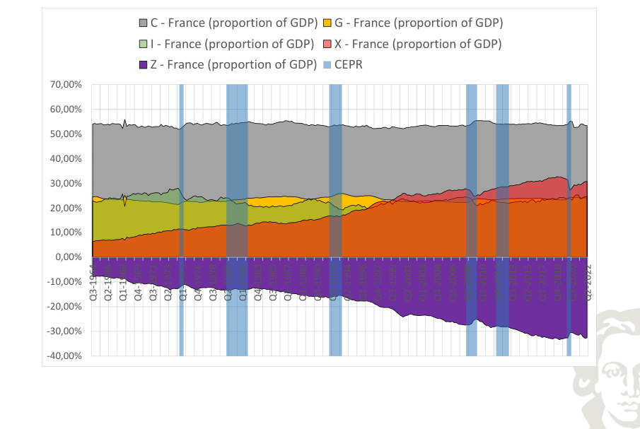
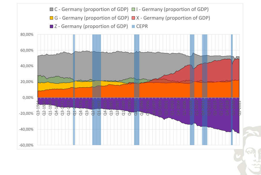
GDP Ratios
Expenditure components can be expressed relative to GDP to compare their importance across time and economies:
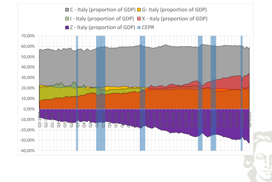
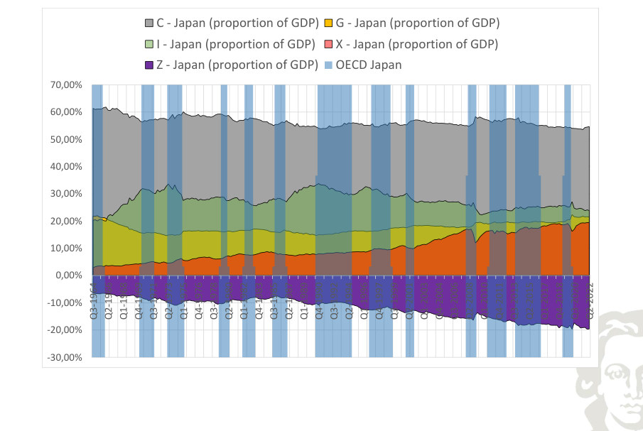
Some aggregate expenditure ratios are relatively stable over long horizons. The country plots use OECD data.
C - United States (proportion of GDP) G - United States (proportion of GDP)
Fit to text
Scroll horizontally to inspect the labels and values.
C - Euro area (proportion of GDP) G - Euro area (proportion of GDP)
Fit to text
Scroll horizontally to inspect the labels and values.
C - France (proportion of GDP) G - France (proportion of GDP)
Fit to text
Scroll horizontally to inspect the labels and values.
C - Germany (proportion of GDP) I - Germany (proportion of GDP)
Fit to text
Scroll horizontally to inspect the labels and values.
C - Italy (proportion of GDP) G- Italy (proportion of GDP)
Fit to text
Scroll horizontally to inspect the labels and values.
C - Japan (proportion of GDP) G - Japan (proportion of GDP)
Fit to text
Scroll horizontally to inspect the labels and values.
Kaldor Stylized Facts
Balanced growth concerns stable long-run ratios and trends, whereas cyclical statistics describe deviations around those trends. Both are useful targets for a quantitative economic model, but they should not be conflated.
A volatility statistic summarizes the typical amplitude of fluctuations; a correlation describes direction and timing of comovement. Dividing a variable's standard deviation by output's standard deviation produces a scale-free relative volatility. Comparing those moments for simulated and observed data provides a model-diagnostic rather than a proof of causality.
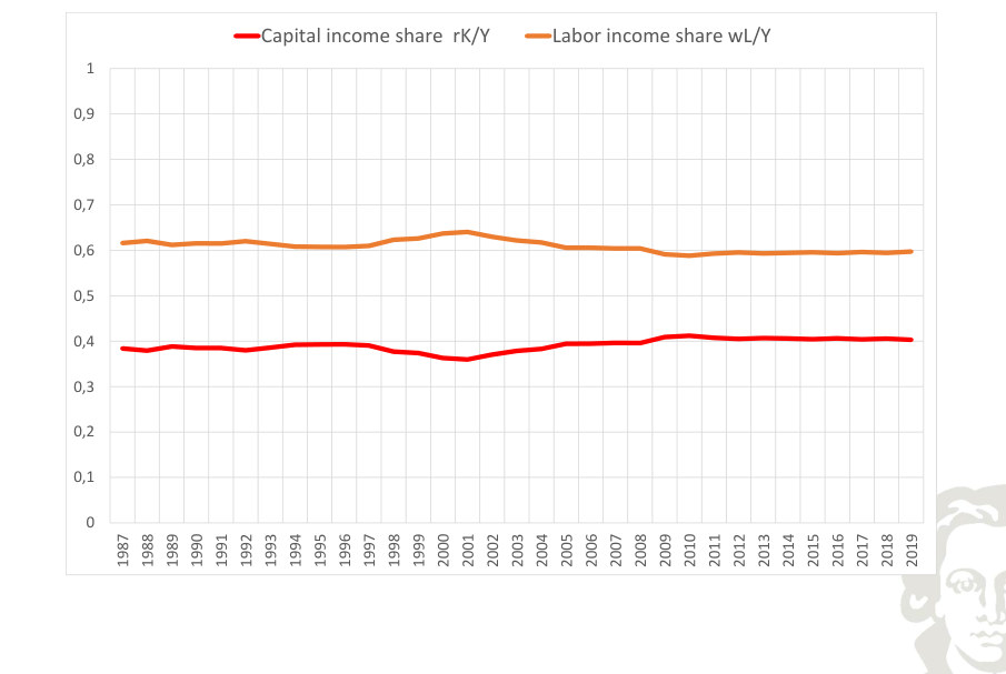
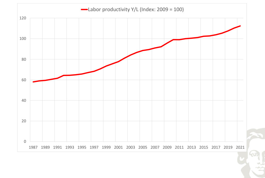
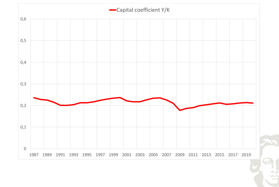
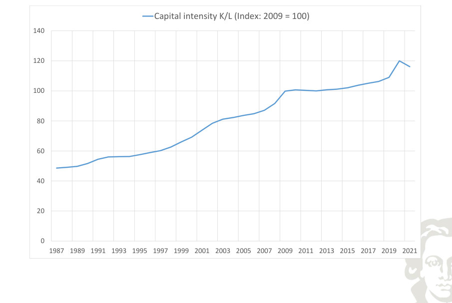
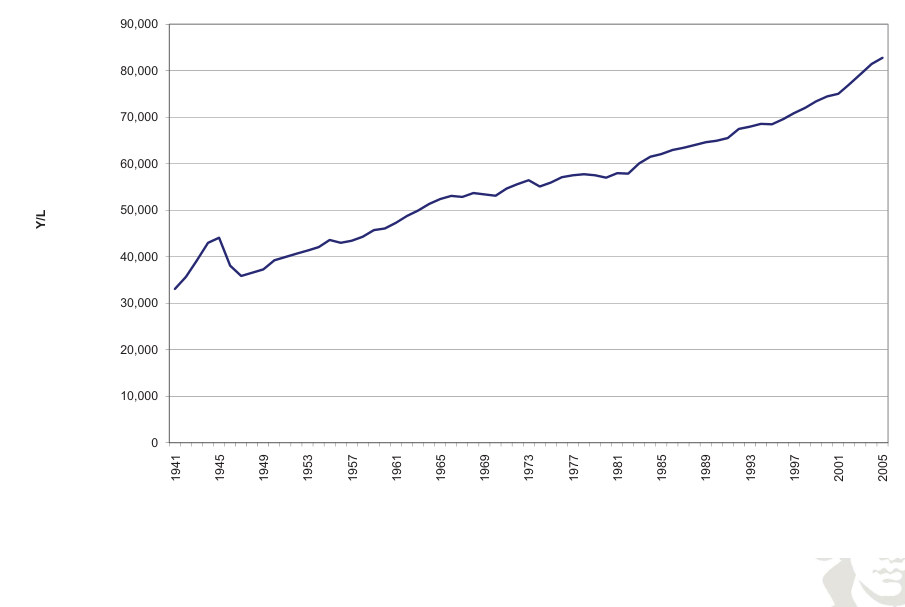
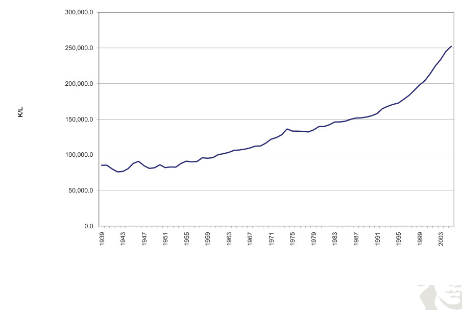
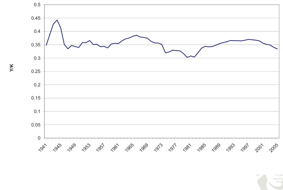
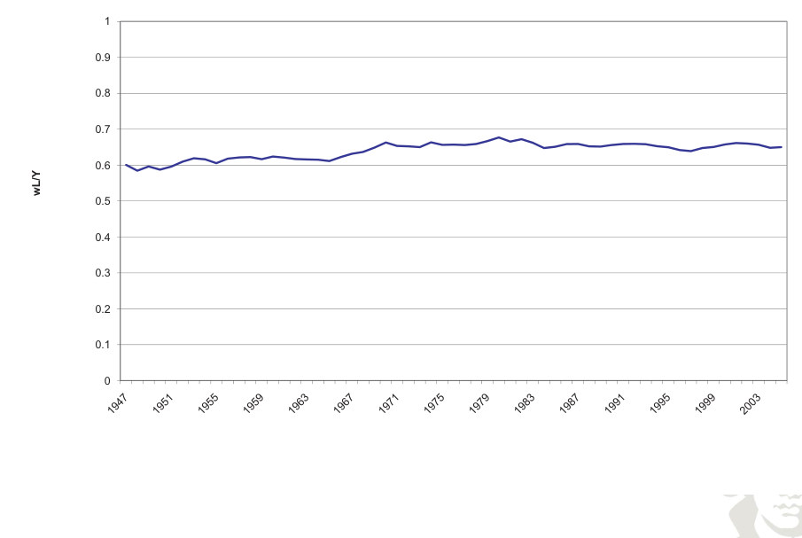
Kaldor’s balanced-growth regularities concern rising output per worker Y/L and capital per worker K/L, a comparatively stable return on capital, a comparatively stable capital–output ratio K/Y, and comparatively stable labor and capital income shares wL/Y and rK/Y. These are long-run regularities rather than exact laws for every sample.
Capital income share rK/Y Labor income share wL/Y
Fit to text
Scroll horizontally to inspect the labels and values.
Labor productivity Y/L (Index: 2009 = 100)
Fit to text
Scroll horizontally to inspect the labels and values.
Capital coefficient Y/K
Fit to text
Scroll horizontally to inspect the labels and values.
Capital intensity K/L (Index: 2009 = 100)
Fit to text
Scroll horizontally to inspect the labels and values.
90,000
Fit to text
Scroll horizontally to inspect the labels and values.
300,000.0
Fit to text
Scroll horizontally to inspect the labels and values.
5
Fit to text
Scroll horizontally to inspect the labels and values.
1
Fit to text
Scroll horizontally to inspect the labels and values.
Solow Model
Capital accumulation creates an intertemporal trade-off: resources devoted to investment raise future productive capacity but reduce resources left for present consumption. In the Solow model the saving fraction is imposed; a steady-state capital stock balances depreciation and effective-labor growth against investment. The Golden Rule savings rate maximizes steady-state consumption, but a structural policy analysis should allow individuals to adjust their saving behavior.
The Solow model expresses output per effective worker as y = k^θ. On its balanced growth path, k and y are constant, while output and capital per worker grow at the rate of labor-augmenting technical progress.
| Quantity | Balanced-growth behavior |
|---|---|
| K/(AL) | Constant |
| Y/(AL) | Constant |
| K/L and Y/L | Grow with A |
| L | Grows with population |
| K and Y | Grow with effective labor AL |
| Y/K | Constant |
In discrete time the gross growth factor of aggregate capital and output is (1+g_A)(1+g_L). The sum g_A+g_L is a first-order approximation. Source: Blanchard and Illing, Macroeconomics, balanced-growth discussion.
Companies
Competitive firms hire capital and labor until their marginal products equal factor prices. With labor-augmenting Cobb–Douglas technology:
A constant capital-to-effective-labor ratio implies a constant capital rental return along the balanced growth path.
Kaldor Facts 5
Competitive Cobb–Douglas factor prices imply labor income wₜLₜ/Yₜ = 1−θ and capital income rₜKₜ₋₁/Yₜ = θ. These constant shares follow from the Cobb–Douglas elasticities together with marginal-product pricing. Constant returns and competition alone imply that factor payments exhaust output; they do not imply constant individual shares for every production function.
Critical Appraisal Of Solow
The Solow model explains growth and capital transition dynamics with an imposed saving rate. It cannot determine how optimal saving changes when taxes, returns or expectations change, because it lacks a household intertemporal optimization problem. This limitation concerns endogenous forward-looking behavior, not the absence of dynamics: the capital accumulation equation is itself dynamic.
Forward-looking households may increase current consumption when they anticipate higher future resources. A model with intertemporal optimization can explain how such expectations influence present saving and consumption.
Decomposing observed macroeconomic data
Data Transformations
Average hours equal total hours divided by employment; labor productivity equals real output divided by hours. A capital series can be built from investment and a stated initial stock using the perpetual-inventory equation:
The initial stock can be independently measured or approximated by i₀/δ under a no-growth steady-state assumption. With Cobb–Douglas production, the log productivity residual is:
The illustrative data construction uses δ = 0.03 and a labor-income share near 0.67. These choices differ from the later benchmark calibration and must remain tied to their respective empirical exercise.
Variability And Correlation
The empirical volatility table above reports log per-capita HP-filtered deviations. Consumption is less volatile than output, while investment is substantially more volatile. Ratios are based on unrounded source moments; dividing the displayed rounded standard deviations may not reproduce every ratio exactly.
Correlation
Empirical cross-correlations of log per-capita HP deviations, corr(Yₜ, xₜ₊ⱼ):
| Series | -3 | -2 | -1 | 0 | 1 | 2 | 3 |
|---|---|---|---|---|---|---|---|
| Output | 0.369 | 0.581 | 0.776 | 1.000 | 0.776 | 0.581 | 0.369 |
| Non-durable consumption | 0.109 | 0.298 | 0.564 | 0.701 | 0.494 | 0.356 | 0.195 |
| Investment | 0.365 | 0.553 | 0.719 | 0.889 | 0.733 | 0.538 | 0.339 |
| Capital | -0.260 | -0.155 | -0.018 | 0.155 | 0.370 | 0.535 | 0.645 |
| Total hours | -0.086 | 0.055 | 0.229 | 0.429 | 0.626 | 0.881 | 0.786 |
| Employment | -0.143 | -0.039 | 0.107 | 0.288 | 0.478 | 0.801 | 0.721 |
| Average hours | 0.333 | 0.512 | 0.678 | 0.772 | 0.684 | 0.581 | 0.414 |
| Labor productivity | 0.136 | 0.049 | -0.065 | -0.244 | -0.418 | -0.475 | -0.500 |
| TFP | 0.471 | 0.627 | 0.753 | 0.875 | 0.550 | 0.301 | 0.055 |
Contemporaneous consumption, investment and TFP are strongly positively correlated with output in this sample. Lead–lag patterns differ across variables.
Synthesis
A model should reproduce clearly defined growth and cyclical facts using appropriately transformed, comparable economic series.
4. The Real Business Cycle model: the firm
Introduction
The RBC economy features optimizing households and firms trading output, labor services and capital services in competitive markets. Firms hire inputs after observing available technology and choose quantities until each factor's marginal product equals its competitive rental price.
The standard production function has Cobb–Douglas form. Its exponent on capital determines the capital income share, and its exponent on labor determines the labor income share when markets are competitive and production has constant returns to scale. Because current output uses the predetermined capital stock inherited from the preceding period, new investment first affects productive capacity in a later period.
Productivity changes are represented by an autoregressive process. Persistence matters: a temporary technological innovation can influence a sequence of future periods, causing households to adjust consumption and investment immediately in anticipation of the future.
Integrated theoretical explanation
The competitive RBC economy consists of a representative household and a representative firm. Firms transform labor services and installed capital services into a final good. Households supply labor, own capital and receive factor income and any distributed profits; they allocate the final good between consumption and investment. In the benchmark closed economy there is only one produced good and no government sector, so aggregate output must equal the resources absorbed by consumption and investment. These simplifying assumptions make the intertemporal mechanism transparent and allow every market-clearing condition to be written precisely.
The firm produces according to yₜ = zₜ kₜ₋₁^α nₜ^(1−α). The variable zₜ is total factor productivity, nₜ is current labor input, and kₜ₋₁ is capital already installed at the start of period t. The exponent α lies between zero and one. Since the exponents add up to one, increasing capital and labor by the same proportion increases output by that proportion; this is constant returns to scale. It does not mean that output grows linearly in one input when the other is held fixed: diminishing marginal productivity with respect to each single input remains present.
A competitive firm takes the real wage wₜ and capital rental rate rₜ as given and maximizes profit, yₜ − wₜnₜ − rₜkₜ₋₁. Differentiating output with respect to labor gives the marginal product of labor (1 − α)yₜ/nₜ, so the optimal labor demand condition is wₜ = (1 − α)yₜ/nₜ. Differentiating with respect to capital gives αyₜ/kₜ₋₁, so rₜ = αyₜ/kₜ₋₁. These are marginal-product pricing conditions, not identities that hold under arbitrary market structure. Under perfect competition and constant returns to scale, payments to labor and capital exhaust output in the benchmark.
The timing convention is economically significant. Capital kₜ₋₁ can be used immediately because it already exists when the period begins, whereas investment selected during period t only contributes to installed capital kₜ and thus to subsequent production. Labor can respond during the current period once the wage and productivity are observed. Confusing kₜ with kₜ₋₁ would alter the model's state structure and can produce incorrect impulse responses, because it would permit today's investment to be used prematurely as today's productive capital.
The productivity state has a stochastic law of motion ln zₜ = ρ ln zₜ₋₁ + uₜ. The innovation uₜ is the newly arriving surprise, while zₜ incorporates the persistent effects of previous surprises. If 0 < ρ < 1, a one-time positive innovation raises current productivity and then decays in expectation at rate ρ. A ρ near one implies a long-lived disturbance; a ρ near zero implies rapid reversion to the normalized steady-state level. Knowing the transition rule and the distribution of innovations enables households to form rational expectations about future productivity.
A favorable technology disturbance shifts the production function outward, raising output for given inputs and increasing the marginal products of capital and labor. Its general-equilibrium effect is more complicated than this direct production shift because higher wages and returns induce households to change hours, consumption and investment. The firm block supplies the demand side of those factor markets, but it does not determine employment or capital accumulation by itself. Those outcomes emerge only after combining factor demand with optimal household decisions, resource feasibility and the shock process.
Formal framework and essential relationships
Current output depends on contemporaneous labor, inherited capital and productivity. The no-growth normalization sets labor-augmenting trend A to one; it does not eliminate stochastic productivity z.
Firms take real wage w and capital rental rate r as given. The decision is static once z and prices are known, although capital is predetermined at the aggregate level.
Under competitive factor demand, each price equals its marginal product. Consequently, wage income is (1−α) of production and gross capital rental income is α of production.
The shock innovation u is not identical to total technology z: z includes the accumulated effects of persistent past innovations. When 0 < ρ < 1, the expected effect decays geometrically.
Explanations, derivations and empirical applications
The economy and its market structure
The competitive conditions and the timing of installed capital jointly determine factor demand. Current technology affects marginal products immediately, whereas investment changes productive capacity only after the installation period.
Productivity disturbances and production
Real Business Cycle Model
A standard RBC economy combines optimizing households and firms with perfectly competitive markets. Households determine consumption, investment and labor supply, while firms demand inherited capital and contemporaneous labor to maximize profit. Aggregate productivity evolves stochastically. The objective is to determine whether productivity innovations transmitted through these optimizing decisions can account for the main observed patterns of aggregate fluctuations.
How the RBC model extends the Solow framework
The RBC framework makes productivity stochastic and allows households to choose consumption, saving and labor supply. The basic Solow model instead imposes a saving rate and labor path.
Goods
Three markets connect households and firms: a final good used for consumption or investment, labor services supplied by households, and capital services supplied by households. Households receive factor income from firms and use it to finance consumption and accumulation. Firms combine the services into output, and the quantities supplied and demanded must coincide at equilibrium prices.
Market Structure
All three markets are perfectly competitive in the benchmark. Individual agents treat the real wage, capital rental rate and final-good price as given, and no firm possesses market power over factor prices or output. This assumption yields marginal-product conditions that allow factor prices to be eliminated from the equilibrium system. It is a modelling simplification whose usefulness depends on the question under investigation.
Information Structure
The period’s productivity state is known when labor and production decisions are made, while the next innovation remains uncertain. Installed capital is inherited from the previous period. Rational expectations require households and firms to use the stochastic structure of the model consistently when anticipating future prices, productivity and returns. Their forecasts need not be perfect, but they must reflect the information and probabilities specified by the model.
Model Environment
The benchmark economy is closed, contains a representative firm and household, and has a single final output good. Firms rent capital and hire labor, while households own the productive assets, supply time and choose consumption and saving. The exclusion of government demand, external trade and nominal rigidities makes the central RBC propagation mechanism easier to trace, but it also restricts which policy questions the model can answer.
Elements Of A Competitive Equilibrium
Households own time, capital and firms; receive wages, capital rental income and profits; and choose labor, investment and consumption to maximize utility. Firms hire labor and capital to maximize profit. Market clearing determines wages and rental rates and requires the goods allocation to satisfy the resource constraint.
Stochastic Production
Production combines a labor-augmenting trend Aₜ and stochastic total factor productivity zₜ.
What Is An AR(1)-Process?
An AR(1) process relates the current value to one lag and a new innovation. The innovation has zero mean, constant variance and is independent across dates. The coefficient ρ measures persistence; covariance stationarity requires |ρ| < 1.
Example AR(1)-Process
Let x₋₁ = 0, set u₀ = 1 and all later innovations to zero. Then:
With ρ = 0.9 the response in period 4 is 0.6561. For |ρ| < 1 it decays to zero.
Fit to text
Scroll horizontally to inspect the labels and values.
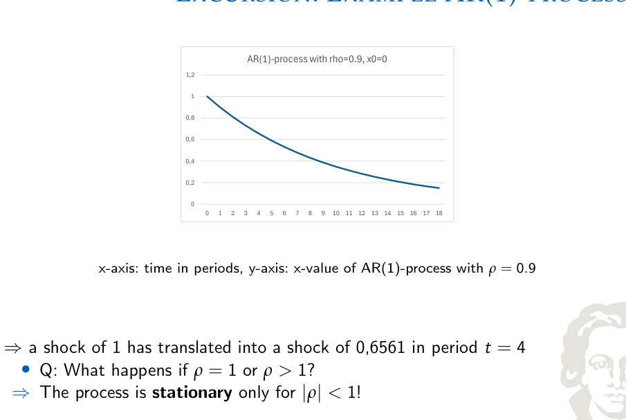
Effect Of Productivity Shocks
An AR(1) process describes persistence with a first-order lag: today's state depends on yesterday's state plus a new innovation. If the persistence parameter lies between zero and one, a positive surprise gradually fades; if it is near one, the disturbance remains influential for many periods. Rational expectations use the probability distribution implied by the model and available information, not perfect foresight.
The stationary mean of log productivity is zero. Its deterministic steady-state level is therefore one. A zero mean of log productivity does not, in general, imply that the stochastic mean of productivity itself equals one.
At fixed labor and inherited capital, zₜ above one raises output relative to the deterministic benchmark; zₜ below one lowers it. This comparison is a level effect at given inputs, not a claim about the unconditional mean of output.
Productivity And RBC
The model describes propagation—the sequence of changes in output, hours, consumption and investment following a productivity innovation—and amplification, the size of those changes relative to the initial shock. Its solution consists of dynamic decision rules and impulse response functions.
Technology: Simplification
Set the labor-augmenting trend Aₜ to one to focus on stationary business-cycle deviations.
Constant Returns To Scale?
Scaling capital and labor by a positive common factor q scales output by q:
The technology has constant returns to scale. Competitive factor payments therefore exhaust output.
Profit Maximization By The Firm
The wage and rental conditions are found by differentiating the profit objective separately with respect to labor and capital. Factor shares exhaust output only because the Cobb–Douglas technology has constant returns and inputs receive their competitive marginal products.
Competitive firms take wages and capital rental rates as given. They choose the input quantities that maximize output value less labor and capital costs.
At given factor prices, substitute the production constraint into profits:
An individual firm chooses rented input services; the aggregate stock available for rental is predetermined.
These marginal-product conditions imply rₜkₜ₋₁ + wₜnₜ = yₜ. Productivity affects wages and rental income through both technology and the equilibrium allocation.
Synthesis
Competition and Cobb–Douglas production connect wages and capital returns to marginal products; productivity is an exogenous persistent state.
5. The representative household and competitive equilibrium
Introduction
In the household block, a representative agent chooses consumption, investment and time devoted to paid work. Leisure provides direct utility but forgoing an hour of work sacrifices wages that could finance consumption. Saving provides tomorrow's productive capital but requires resources to be withheld from consumption today.
Dynamic optimization generates two economically distinct equilibrium conditions. The Euler equation balances the marginal utility of consuming today against the discounted expected benefit of investment and future consumption. The intratemporal labor condition compares the marginal utility of leisure with the wage measured in utility units.
Firm optimality, household optimality, market clearing and the economy-wide resource constraint are all needed for competitive equilibrium. A condition derived for one agent is not sufficient: all desired factor purchases and supplies must agree, and aggregate expenditure cannot exceed production.
Integrated theoretical explanation
The representative household begins with a stock of installed capital and a normalized time endowment of one unit each period. Time is divided between labor nₜ and leisure ℓₜ, so nₜ + ℓₜ = 1. Working more hours generates wage income but removes leisure; retaining more current output for consumption reduces the resources that can finance investment. The household's decisions therefore combine an intratemporal trade-off between consumption and leisure and an intertemporal trade-off between consumption today and consumption in the future.
Lifetime utility takes the form E₀Σβᵗu(cₜ,ℓₜ), where β between zero and one discounts future utility and E₀ represents expectations given information available at the initial date. A general family of consumption–leisure preferences can be specialized to logarithmic consumption and linear utility from leisure, u(c,ℓ) = ln c + ϕℓ. Under this specification, the marginal utility of consumption equals 1/c and the marginal utility of leisure is the constant ϕ. Concavity in consumption makes a more evenly distributed consumption path preferable to large fluctuations with the same average level.
The household faces a budget restriction that combines the wage bill, the rental income earned on installed capital, distributed profits and undepreciated capital. Writing next-period productive capital on the spending side, cₜ + kₜ = wₜnₜ + rₜkₜ₋₁ + πₜ + (1 − δ)kₜ₋₁, expresses the use of all available resources when the optimum is interior. This is equivalent to accounting for investment separately with kₜ = (1 − δ)kₜ₋₁ + iₜ. The depreciation rate δ measures the fraction of old capital physically lost between periods.
The Euler equation is the condition for optimal saving. Sacrificing one unit of consumption in period t gives up current marginal utility 1/cₜ but increases capital available for the next period. That capital produces rental income rₜ₊₁ and retains the undepreciated fraction 1 − δ. The expected future payoff must therefore be discounted and weighted by marginal utility at t+1. At an interior optimum, 1/cₜ = βEₜ[(rₜ₊₁ + 1 − δ)/cₜ₊₁]. If the expected return rises, households generally have an incentive to save more, although the total response also depends on wealth and future income expectations.
The intratemporal first-order condition compares the utility lost from less leisure with the utility gained from wage-financed consumption. Under the specified utility function, ϕ = wₜ/cₜ, or equivalently ϕcₜ = wₜ. Combining this with competitive labor demand yields ϕcₜ = (1 − α)yₜ/nₜ. The equation does not say that households supply a fixed number of hours: it makes labor supply jointly dependent on consumption, productivity and the equilibrium wage. A change in labor productivity alters the wage opportunity cost of leisure and therefore the desired allocation of time.
Consumption smoothing and labor adjustment interact following a technology shock. Higher current productivity provides more goods and raises the potential return on capital. Forward-looking households need not consume all extra production immediately: saving part of it supports consumption in later periods when the technology shock has diminished. At the same time, higher real wages affect the relative attractiveness of leisure and work. A consistent equilibrium determines both margins together; one cannot infer the labor response from the firm's marginal-product equation alone or the consumption response from a budget identity alone.
A competitive equilibrium is a sequence of allocations, factor prices and expectations for which households maximize utility subject to their constraints, firms maximize profits, markets clear, capital follows its accumulation law and productivity follows its exogenous process. Under the closed-economy benchmark, the goods market requires yₜ = cₜ + iₜ. The capital-service and labor markets equate household supply with firm demand. Inserting the competitive factor-price equations into household optimality reduces the model to a compact set of dynamic equations for y, c, n, k and z, which is the starting point for calibration and solution.
Formal framework and essential relationships
The household utility is specialized to logarithmic consumption and linear leisure. The discount factor β determines the weight on future utility; ϕ governs the marginal utility of leisure. Each time endowment is normalized to one.
Consumption plus investment in next period’s productive capital is financed by wages, capital rental income, profits and undepreciated old capital.
Euler/Lucas asset-pricing equation. Investing one resource unit sacrifices 1/cₜ units of marginal utility today and yields a random gross payoff tomorrow. Equality characterizes an interior optimum.
At the intratemporal optimum, the marginal disutility from additional working time balances the real wage valued at the marginal utility of consumption; the second equality clears the labor market.
In the benchmark closed economy with neither public expenditure nor external trade, all output is allocated to consumption or gross investment. Combining this identity with capital accumulation yields the aggregate resource constraint.
Explanations, derivations and empirical applications
Endowments
Household optimization allocates resources across consumption, saving and leisure. The Euler equation and the labor–leisure condition are necessary restrictions that must hold simultaneously with market clearing and the feasible resource allocation.
Households enter the first period with installed productive capital and receive one unit of time in each period. They divide time between working hours and leisure, imposing 1 = nₜ + ℓₜ. Labor produces wage income, whereas leisure yields direct satisfaction but no production. The inherited capital stock finances rental income and provides a state variable linking past investment choices to current consumption opportunities.
Preferences
The preference function must make consumption and leisure desirable and satisfy concavity restrictions. For the non-logarithmic form, restrictions on v and its derivatives depend on σ; marginal-sign conditions alone do not establish joint concavity. The benchmark specializes to:
Why This Utility Function?
Balanced-growth-compatible preferences restrict how consumption and leisure enter utility. Logarithmic consumption with separable leisure is a useful special case: it permits consumption and real wages to grow while hours remain stationary under suitable technology and equilibrium conditions. It is a member of a broader family of preferences, not the uniquely possible utility function.
Rational Expectations
Rational expectations mean that decisions are based on the conditional probability distribution implied by the model and all information available at the decision date. They do not imply that agents know future innovations. Rather, expectations are mathematically consistent with the economy’s stated technology process, equilibrium prices and decision rules. This requirement is indispensable for interpreting the Euler equation in a stochastic environment.
Household’s Optimization Problem
The household takes initial capital as given. Feasibility, nonnegativity and an appropriate transversality condition complement the interior first-order conditions.
First-order condition for capital
Capital chosen at t appears as a cost at t and earns rental income plus an undepreciated remainder at t+1. Differentiating both appearances gives:
Only current information is available when the future payoff is evaluated.
Optimal Capital Supply
The choice of next-period capital equates the utility cost of sacrificing consumption today with the discounted expected utility value of the gross return tomorrow. That return includes the capital rental payment and the undepreciated remainder of the asset. With logarithmic consumption utility, the resulting Euler equation can be expressed as 1/cₜ = βEₜ[(rₜ₊₁ + 1 − δ)/cₜ₊₁].
Household Optimization: Intuition
The marginal utility cost of less current consumption equals the discounted expected utility benefit of future capital returns. The future rental return depends on the future technology realization and allocation:
If the discounted expected marginal utility benefit of saving exceeds its current utility cost, the household can improve utility by investing more. If the inequality is reversed, it can improve utility by consuming more now. An interior optimum equates the two sides of the Euler condition.
Abstracting from expectations for a second, we can uncover a little more intuition.
In a deterministic environment, intertemporal optimality equates willingness to exchange current for future consumption to the feasible gross return:
The left side is the intertemporal marginal rate of substitution; the right side is the marginal rate of transformation. Under uncertainty, the Euler equation uses the conditional expected utility-weighted return.
Consumption Smoothing: Intuition
Smoothing follows from concave utility, not from a rule that consumption must literally stay constant. Expected increases in lifetime resources can raise consumption immediately, while the stock of capital absorbs much of the short-run variation in saving.
Concavity creates a preference for smoother consumption, conditional on lifetime resources, relative prices, uncertainty and borrowing opportunities. It does not require consumption to be constant.
A favorable productivity realization, zₜ above its reference level of one, raises output for given inputs. If labor does not fall enough to offset this effect, the additional output must be absorbed by consumption, investment or both.
As agents want to smooth consumption, they want to spread the increase in output over multiple periods. In other words, they don’t want to consume the entire increase ∆ct < ∆yt; Hence, agents want to invest a portion of the increased output ∆it > 0, as investment postpones consumption to the future.
Consumption Smoothing: Propagation
An impulse response is a controlled thought experiment rather than a historical forecast. The only new shock arrives initially; subsequent responses reflect the model's internal propagation. Capital is predetermined at the start of a period, while employment and consumption may adjust contemporaneously. Simulation repeats this mechanism over many random shocks to generate model-implied moments.
1 Positive technology shock increases output ∆yt; 2 Due to their desire to smooth consumption, investment increases ∆it > 0; 3 This increases the capital stock for tomorrow ∆kt = ∆it; 4 and so output in the future increases; 5 return to step 1).
But: we haven’t shown that labor nt reacts such that output indeed increases in response to a positive technology shock (usually it does, though).
Optimal Labor Supply
The consumption–leisure condition translates a preference trade-off into a market equation. Under logarithmic consumption and linear leisure it becomes ϕcₜ = wₜ, which must be solved jointly with the firm’s marginal product of labor.
Working an additional unit of time reduces leisure by one unit and increases the household’s available consumption by the real wage. With utility ln c + ϕℓ, the marginal utility loss from less leisure is ϕ and the consumption gain has utility value w/c. The intratemporal optimum therefore satisfies ϕcₜ = wₜ. Market clearing then replaces wₜ by the marginal product of labor.
Household Optimization: Intuition
Working one additional unit of time trades off lost leisure against wage-financed consumption. At an interior optimum:
If ul (ct, lt) < uc (ct, lt) · wt the utility gain from additional consumption financed through more work is greater than the utility loss of forgone leisure. Therefore, the household can increase its level of utility by working more and consuming from the additional income.
If however ul (ct, lt) > uc (ct, lt) · wt the utility gain from additional leisure is greater than the utility loss of forgone consumption financed through more work. Therefore, the household can increase its level of utility by working less and enjoying more leisure. So as long as the equality does not hold, it is possible for the household to increase its welfare by adjusting its labor-leisure choice.
The marginal rate of substitution between leisure and consumption equals the real wage, the market’s marginal rate of transformation between the two.
Labor Supply: Propagation
A higher wage creates opposing effects on labor supply. The substitution effect makes leisure more expensive and encourages work; the income effect makes the household wealthier and can increase desired leisure. Their balance depends on preferences, persistence and equilibrium prices. Under the benchmark calibration, hours increase after a positive technology innovation.
If households respond to wt ↑with more labor nt ↑, then the effect of technology shocks increases: Output increases further than with the technology shock alone (amplification). This output increase is only partially consumed: investment increase and so forth following from the consumption smoothing motive.
Market Clearing
Goods, labor and capital markets must clear simultaneously. Total production is absorbed by consumption and investment, labor supplied equals labor hired, and the capital stock rented to firms is the stock owned by households. When firm profits are distributed back to their owners, household budgets are consistent with the aggregate resource identity. These restrictions convert individual optimal decisions into a competitive equilibrium.
Equilibrium
An equilibrium is a situation in which (A) households maximize, (B) firms maximize, (C) markets clear, (D) households form expectations rationally.
Market Clearing I: Labor Market
Market Clearing II: Capital Market
Resource Constraint
Under constant returns and competitive pricing, profits are zero and factor payments exhaust production. Monotonic preferences make the household’s resource constraint bind at equilibrium.
Summary
The nonlinear equilibrium system consists of the Euler condition, labor-market condition, resource constraint, production function and technology process:
Synthesis
Consumption, saving and labor decisions derive from household optimality. Equilibrium requires jointly satisfied Euler, labor, production and resource conditions.
6. Steady state, calibration and log-linear approximation
Introduction
A nonlinear RBC model is an internally consistent system of forward-looking difference equations, but it is not usually convenient to study directly by hand. The solution follows a standard sequence: identify the deterministic steady state, assign parameter values, approximate equilibrium conditions in log deviations and solve the resulting linear system.
The steady state gives a reference point. Calibration links structural parameters to empirical moments and equilibrium identities rather than selecting values without justification. Log-linearization then measures small percentage departures from this point; its quality must be judged relative to the size of the shocks being analyzed.
A first-order approximation preserves local effects but loses genuinely nonlinear features of large excursions, occasionally binding constraints and precautionary behavior. Thus the model's first-order impulse responses are most informative for small disturbances around the calibrated steady state.
Integrated theoretical explanation
The complete benchmark RBC system contains five central relationships. The Euler condition connects consumption today with expected consumption and capital returns tomorrow. The labor condition links consumption and hours to the marginal product of work. The resource constraint allocates output between consumption and capital accumulation. The production function determines goods available from productivity, labor and inherited capital. Finally, the autoregressive technology process describes how new innovations alter the exogenous state. Solving the model means finding paths that satisfy all five equations simultaneously, not solving each in isolation.
A deterministic steady state is a constant configuration of the endogenous variables in an environment without further technology innovations. Productivity is normalized to one. Because capital no longer changes from period to period, the investment required merely replaces the amount depreciated, so ī = δk̄. The steady-state resource restriction is ȳ = c̄ + δk̄. The Euler equation yields 1 = β[αȳ/k̄ + 1 − δ], which identifies the required steady-state marginal product of capital as αȳ/k̄ = β⁻¹ − 1 + δ. These are equilibrium restrictions rather than independent numerical assumptions.
The capital–output ratio follows immediately from the required return: k̄/ȳ = α/(β⁻¹ − 1 + δ). Because investment just replaces depreciation, the steady-state investment share satisfies ī/ȳ = δ(k̄/ȳ). Consumption's output share is then c̄/ȳ = 1 − δ(k̄/ȳ). Given a normalization for hours n̄ and the Cobb–Douglas technology, the level of steady-state output is pinned down by these ratios. The leisure-preference parameter ϕ can be chosen so that the labor first-order condition holds at the target steady-state hours. Working through these steps in order avoids attempting to solve simultaneously for every unknown without using the identifying equilibrium relationships.
Calibration means using the structure of the model and observed economic magnitudes to choose plausible parameter values. The capital share α is associated with the observed share of income paid to capital when factor prices equal marginal products. Depreciation is informed by the pace at which productive assets wear out; β is linked to the equilibrium capital return; ϕ helps match average hours; ρ characterizes technology persistence; and the innovation standard deviation controls shock size. A calibrated value does not become a universal economic constant: it is a choice connected to a dataset, frequency, production structure and target moments.
The Solow residual is a measure of total factor productivity inferred from output and measured factor inputs. Taking logs of Cobb–Douglas production produces ln zₜ = ln yₜ − α ln kₜ₋₁ − (1 − α)ln nₜ. Its construction assumes that the production elasticity and input series are appropriately measured. The residual may also contain variation caused by utilization, composition, omitted inputs or measurement error. Treating every movement in the measured residual as a pure exogenous technology shock is a strong interpretation, and the empirical implications of the RBC framework should be assessed with that limitation in mind.
Linearizing around a steady state is useful because the original equilibrium conditions contain nonlinear products, powers, ratios and expectations. For a strictly positive variable, define x̂ₜ = ln(xₜ/x̄). A small x̂ₜ is approximately the proportional deviation (xₜ − x̄)/x̄. The approximation takes advantage of exp(x̂ₜ) ≈ 1 + x̂ₜ near zero. In logarithms, Cobb–Douglas production has an exact linear representation, ŷₜ = ẑₜ + (1 − α)n̂ₜ + αk̂ₜ₋₁. Other equations require a first-order Taylor expansion because their level expressions contain sums or more complicated nonlinearities.
The goods-market resource identity provides a particularly important example. Begin with yₜ = cₜ + kₜ − (1 − δ)kₜ₋₁ and express every positive variable as its steady-state level multiplied by exp of its log deviation. Keeping first-order terms and cancelling the steady-state identity gives ȳŷₜ = c̄ĉₜ + k̄k̂ₜ − (1 − δ)k̄k̂ₜ₋₁. The weights are steady-state levels; they cannot be omitted simply because the model has been written in percentage deviations. Dividing by ȳ converts the equation into ratios that can be interpreted as resource shares.
For the labor condition, ϕcₜ = (1 − α)yₜ/nₜ, take logarithms and subtract the steady-state equation. All fixed constants cancel, leaving ĉₜ = ŷₜ − n̂ₜ. The familiar condition that real wages equal the marginal product of labor produces the same percentage logic. For the technology process, the log law of motion is already linear. The Euler equation is more delicate because it contains a conditional expectation of a future product and must be expanded jointly around steady-state consumption and returns. The resulting system is linear in state and control deviations but retains forward-looking expectations.
A first-order approximation is reliable only locally. It describes the immediate marginal effect of small changes around the calibrated reference point, not necessarily the response to very large crises, irreversible investment constraints or nonlinear regime changes. Its main advantage is that a complicated dynamic optimization model can be studied using a system of linear rational-expectations difference equations. Once solved, that linear system yields policy functions, impulse responses and model-generated statistics that can be compared systematically with business-cycle data.
Formal framework and essential relationships
With no growth and no innovations, the Euler equation equates discounting to the steady-state gross capital return; investment merely replaces depreciation.
The steady-state labor equation and production function jointly determine hours, output, consumption and capital once parameters are chosen.
| Parameter | Illustrative calibration | Economic role |
|---|---|---|
| ρ | 0.95 | Persistence of log technology |
| σᵤ | 0.007 | Standard deviation of productivity innovations |
| α | 0.36 | Capital income share |
| ϕ | 2.56 | Marginal utility weight on leisure |
| δ | 0.0225 | Capital depreciation per quarter |
| β | ≈ 0.99 | Household discount factor |
The calibration uses σ for the standard deviation of innovations, whereas σ denotes utility curvature in the earlier general CRRA specification. The meaning must therefore be inferred from the equation or parameter table under discussion.
A hat denotes a log deviation from steady state, which is approximately a proportional change for small shocks. The approximation exp(h) ≈ 1+h is the local first-order Taylor formula.
The linearized labor and production equations turn nonlinear ratios and products into combinations of deviations with economically interpretable coefficients.
The linearized resource constraint is expressed in units of steady-state quantities, not a simple unweighted sum of percent changes.
Explanations, derivations and empirical applications
Approximating The Solution
The deterministic steady state, structural calibration and approximation are separate stages of the quantitative solution. Together they transform a nonlinear general-equilibrium system into a tractable local description of dynamic responses.
The quantitative procedure proceeds in a fixed logical order: calculate the deterministic steady state, choose calibrated or estimated parameters, log-linearize the nonlinear equilibrium conditions, solve the linear rational-expectations system, and examine the resulting impulse responses. Starting with the steady state is necessary because all first-order coefficients are evaluated at that reference allocation.
Nonlinear System Of Equations
The equilibrium conditions to be calibrated and approximated are:
Steady State
A deterministic steady state removes innovations and holds stationary endogenous variables constant:
Constant consumption removes the intertemporal consumption ratio; the steady-state return offsets discounting.
Investment And Output
With constant capital, investment replaces depreciation.
Steady State Factor Shares
Calibrating The Model
There are 6 parameters in the model to set β, δ, α, ϕ, ρ, σ; Now we will calibrate the model to match several stylized facts. We need a calibration target for each parameter; directly from the data; or the steady state equations.
Calibrating Directly From The Data
Some parameters can be set directly from the data.
The log of the cyclical productivity component can be fitted to an AR(1) process. The illustrative quarterly calibration uses persistence ρ = 0.95 and innovation standard deviation σᵤ = 0.007; these values are calibration choices, not estimates for every economy.
What Are Solow Residuals?
Calibration assigns parameter values using directly observable persistence and shock measures, factor shares, and steady-state accounting identities. For example, competitive Cobb–Douglas production makes the capital exponent equal to capital's income share. Solow residuals attribute the part of output not accounted for by measured input quantities to total factor productivity, which may also include measurement error or omitted factors.
With Cobb–Douglas production, the level of measured productivity is the residual after accounting for capital and labor:
Allowing the measured capital share to vary over time replaces α by αₜ. Interpreting this residual as technology requires assumptions about input measurement, utilization and production structure.
Solow Residuals And Productivity Shocks
Kaldor-style facts are long-run restrictions that help determine whether an aggregate production model is plausible. Balanced growth links rising labor productivity and capital intensity with relatively stable factor proportions, capital returns and income shares. They do not imply a constant output level or that short-run fluctuations are unimportant.
A stochastic productivity process can be approximated by fitting an autoregressive model to the measured productivity residual. The estimated persistence determines how long a typical innovation affects productivity, while the residual innovation dispersion determines shock size. Interpreting the statistical residual as pure exogenous technology remains an identifying assumption of the benchmark RBC model.
Calibration
The capital elasticity is calibrated to the observed capital-income share under the competitive Cobb–Douglas assumptions.
Calibration: Summary
| Parameter | Illustrative value | Calibration basis |
|---|---|---|
| ρ | 0.95 | Persistence of log productivity |
| σᵤ | 0.007 | Innovation standard deviation |
| α | 0.36 | Capital-income share |
| ϕ | 2.56 | Hours and consumption share |
| δ | 0.0225 | Investment share and output–capital ratio |
| β | ≈0.99 | Steady-state Euler condition |
Log Deviations
A log deviation is ln(xₜ/x̄), approximately the percentage difference from the steady-state level when the deviation is small. First-order Taylor expansion turns products and powers into weighted sums of log deviations, greatly simplifying the equilibrium system. It is a local method: when departures become large, approximation errors can be economically material.
For small changes, the log deviation approximates a proportional deviation. Multiplying by 100 gives percentage units.
Example: Log Deviations
Consumption is approximately 2.2% above its reference level. With cₜ = 5.35, the log deviation is approximately −0.01484, or −1.48%.
Loglinearization Around The Steady State
This is a local first-order approximation around zero log deviation.
Example: Loglinearization
How Good Is The Approximation?
The approximation error is about 0.00496, small relative to the change in the function.
The error increases to about 0.46485. Larger departures make the local approximation less accurate.
Loglinearizing
The labor condition is exactly linear in log deviations.
Canceling the steady-state production identity and taking logs gives an exact log relation.
Expand each exponential to first order and subtract the steady-state resource identity:
Unlike the Cobb–Douglas equation, this relation is an approximation.
Expand both exponentials and use the steady-state Euler condition:
Linear System Of Equations
Synthesis
Calibration fixes economically interpretable parameters; first-order approximation translates nonlinear dynamics into a tractable local system.
7. Solving the linear rational-expectations model
Introduction
Solving a forward-looking linear model means finding expectations and decision rules consistent with every equilibrium condition. Unlike a static linear system, arbitrary algebraic solutions are not equally admissible: the selected process must be stable and respect the predetermined state variables.
The method of undetermined coefficients conjectures policy functions linear in the beginning-of-period capital stock and observed technology. Substitution into the log-linearized Euler, labor, production and resource equations identifies coefficient restrictions. The stable root is selected to obtain the economically relevant recursive equilibrium.
The same linear rational-expectations system can be expressed in Harald Uhlig's matrix-based toolkit and implemented numerically in Matlab or Dynare. These computational environments solve for response coefficients, assess dynamic stability and generate model-implied statistical moments.
Integrated theoretical explanation
Log-linear equilibrium equations are not yet a complete economic solution because they include expectations about variables at future dates. A recursive equilibrium expresses current decisions as functions of states known when those decisions are made. In the RBC benchmark, the key states are installed capital from the previous period and the current technology state. Installed capital is predetermined by earlier investment; technology is exogenous but observed within the period. Consumption, hours and the choice of new capital adjust to these states according to decision rules that must satisfy both current and expected future equilibrium conditions.
The method of undetermined coefficients starts by proposing linear policy functions. For example, write k̂ₜ = λkk k̂ₜ₋₁ + λkz ẑₜ, with analogous expressions for consumption, output and labor. The coefficients are initially unknown, but linearity suggests that any stable first-order solution can be represented in this form. These equations have an immediate economic interpretation: one coefficient describes the effect of inheriting an additional unit of capital relative to the steady state; the other describes the effect of a higher productivity state when inherited capital is held fixed.
Substitute the proposed rules into production, the labor condition, the resource constraint and the forward-looking Euler condition. Because the technology state itself obeys ẑₜ₊₁ = ρẑₜ + uₜ₊₁, rational expectations can be computed using the conditional mean of future shocks. Collect all terms involving k̂ₜ₋₁ and all terms involving ẑₜ. For the identities to hold for every possible state combination, each corresponding coefficient must satisfy a separate algebraic restriction. The resulting nonlinear equations in the λ coefficients are solved together, and the economically admissible stable branch is selected.
Stability matters because the model contains a predetermined asset and forward-looking choices. An algebraic root that causes the state vector to explode under small disturbances may violate the transversality conditions of the household problem and fail to describe a reasonable equilibrium around steady state. A stable solution lets the economy converge after temporary shocks when the underlying exogenous process is stationary. This is not merely a preference for smooth-looking graphs: it is the dynamic consistency requirement connecting optimal saving, expected returns and the time path of accumulated capital.
The calibrated decision coefficients make the economic responses concrete. In the reported numerical example, k̂ₜ ≈ 0.95k̂ₜ₋₁ + 0.15ẑₜ, while ĉₜ ≈ 0.53k̂ₜ₋₁ + 0.45ẑₜ and ŷₜ ≈ 0.05k̂ₜ₋₁ + 1.97ẑₜ. Labor responds approximately as n̂ₜ ≈ −0.48k̂ₜ₋₁ + 1.52ẑₜ, and investment has a much stronger technology loading. These are local responses based on the particular calibration, not general coefficients that should be transplanted into any economy.
Uhlig's toolkit provides a matrix representation of the same system. Endogenous state variables, non-state controls and exogenous shocks are separated into vectors. Static equations link contemporaneous and lagged states to controls, while expectational equations include future values. Solving the matrix system produces coefficient matrices P and Q for the endogenous state transition and R and S for the remaining control variables. This approach scales to models with more variables than can comfortably be solved by hand and gives numerical diagnostics, including candidate roots, stability information and model moments.
The practical computer workflow follows the same conceptual sequence as the hand derivation: choose parameter values, calculate the deterministic steady state, declare the ordering of variables, construct equation matrices, verify their dimensions and call the solver. Output matrices must be interpreted against the declared variable order; swapping consumption and investment in a software vector can make otherwise correct numbers economically meaningless. The examples also show how a calibration can be used to obtain autocorrelations and standard deviations after filtering simulated data.
Dynare is an alternative environment for specifying and solving dynamic stochastic general-equilibrium systems. Rather than treating a software package as a source of economic assumptions, the researcher supplies the equations, calibrated or estimated parameters, shock process and requested analyses. The quality of the outcome still depends on whether the equations are correctly timed and whether the steady state and equilibrium structure are coherent. Numerical software is an implementation of a mathematical model, not a substitute for specifying the model or interpreting its results.
Formal framework and essential relationships
The endogenous state evolves according to inherited capital and the current productivity state. Its response coefficients emerge by substituting the conjectured laws into the equilibrium system.
Consumption and output are controls that move immediately in response to the states. Similar equations characterize labor and investment.
| Endogenous variable | Loading on k̂ₜ₋₁ | Loading on ẑₜ |
|---|---|---|
| Capital, k̂ₜ | 0.95 | 0.15 |
| Consumption, ĉₜ | 0.53 | 0.45 |
| Output, ŷₜ | 0.05 | 1.97 |
| Hours, n̂ₜ | −0.48 | 1.52 |
| Investment, îₜ | −1.40 | 6.52 |
The policy-function coefficients are displayed in rounded form for readability. A numerical matrix implementation can report additional decimal places, so minor rounding differences do not indicate a different model.
Uhlig’s solution uses a matrix law for states x and controls y, with exogenous technology z. The transition eigenvalues and estimated matrices show whether the selected equilibrium is stable.
Explanations, derivations and empirical applications
Linear System Of Equations
Method Of Undetermined Coefficients
Installed capital and current productivity are the state variables. Conjecture linear decision rules:
Eliminate output and labor to reduce the model to capital, consumption and technology:
Substitute the conjectured capital and consumption rules and use the conditional expectation of productivity:
Next Steps
The forward-looking consumption rule must be evaluated using next period’s endogenous capital state:
Substitute the capital and consumption rules again, then collect the coefficients on inherited capital and current technology separately.
Comparing Coefficients
Choose the economically admissible stable root. If the absolute product of the two roots exceeds one, at most one can lie strictly inside the unit circle.
These restrictions follow from matching the coefficient on current productivity, independently of the coefficient on lagged capital.
Calibrated policy functions
| Variable | Loading on inherited capital | Loading on productivity |
|---|---|---|
| Capital | 0.95 | 0.15 |
| Consumption | 0.53 | 0.45 |
| Output | 0.05 | 1.97 |
| Hours | −0.48 | 1.52 |
| Investment | −1.40 | 6.52 |
Rounded illustrative coefficients describe local responses in log deviations.
Uhlig’s Toolkit
The matrix representation distinguishes equations that hold within a period from equations that contain expectations of future decisions. This separation allows a general numerical solution with state and control vectors.
The vectors distinguish endogenous states x, other endogenous variables y and exogenous states z. Matrix dimensions and rank conditions must be compatible with the equation and variable counts; the selected solution must respect the predetermined states and stability requirements.
Solution
A stable recursive representation maps predetermined capital and current productivity into optimal control decisions. Its coefficients and matrix roots must satisfy the dynamic equilibrium equations and the timing of endogenous states.
The matrix solution has the recursive form xₜ = Pxₜ₋₁ + Qzₜ for endogenous states and yₜ = Rxₜ₋₁ + Szₜ for other endogenous variables. The matrices summarize how predetermined states and exogenous disturbances determine current allocations. Once they are known, impulse responses and stochastic simulations follow from repeated application of these transition laws.
Log-linearized System Of Equations
Uhlig’s Toolkit
The first block contains labor, resource, production and accumulation equations; the second contains the Euler equation; the final block is the exogenous transition.
Applying The Toolkit
For the four-control representation, the expectational matrices in the Euler block are:
Rows correspond respectively to labor equilibrium, resources, production and capital accumulation; controls are ordered as consumption, output, labor and investment.
Numerical implementation
This implementation adds the gross capital return to the control vector, so its matrices differ in dimension from the four-control representation above. Keep this ordering consistent when interpreting numerical output. The variable named “interest” is the gross return r + 1 − δ.
% Quarterly RBC calibration
alpha = 0.36;
delta = 0.0225;
betta = 0.99;
rho_z = 0.95;
sigma_eps = 0.007;
N_bar = 1/3;
Z_bar = 1;

% Deterministic steady state
R_bar = 1/betta;  % Gross return, rental return plus 1-delta
YK_bar = (R_bar + delta - 1)/alpha;
K_bar = (YK_bar/Z_bar)^(1/(alpha-1))*N_bar;
I_bar = delta*K_bar;
Y_bar = YK_bar*K_bar;
C_bar = Y_bar-I_bar;
phi = (1-alpha)*Y_bar/(N_bar*C_bar);

% State: capital. Controls: consumption, output, labor,
% gross return, investment. Exogenous state: technology.
VARNAMES = char('capital','consumption','output','labor', ...
                'interest','investment','technology');
AA = [0; -K_bar; 0; 0; 0];
BB = [0; (1-delta)*K_bar; alpha; 0; -alpha*YK_bar];
CC = [-C_bar, Y_bar, 0, 0, -I_bar;
       0, 0, 0, 0, I_bar;
       0, -1, 1-alpha, 0, 0;
      -1, 1, -1, 0, 0;
       0, alpha*YK_bar, 0, -R_bar, 0];
DD = [0; 0; 1; 0; 0];
FF = 0; GG = 0; HH = 0;
JJ = [-1, 0, 0, 1, 0];
KK = [1, 0, 0, 0, 0];
LL = 0; MM = 0;
NN = rho_z;
Sigma = sigma_eps^2;
[l_equ,m_states] = size(AA);
[~,n_endog] = size(CC);
[~,k_exog] = size(DD);

% Analysis options for the toolkit
PERIOD = 4;
GNP_INDEX = 3;
IMP_SELECT = 1:7;
DO_SIMUL = 0;
DO_MOMENTS = 1;
HP_SELECT = 1:(m_states+n_endog+k_exog);
% With the toolkit on the MATLAB path, invoke its driver:
% do_it;
The coefficient matrices are reconstructed from the equilibrium equations. The rounded discount factor is set to 0.99, so ratios calculated from the code can differ slightly from calibration targets stated with fewer decimal places.
Calling The Toolkit
In a computational implementation, the researcher must make the model file and solver accessible to the numerical environment, supply the equilibrium matrices and run the routine. The economic content is in the model equations and parameter choices, not in the computer’s directory path. Output should be checked for consistency with the stated variable ordering and for stable roots.
Toolkit Output
The endogenous state is capital; the exogenous state is technology. Candidate transition roots and the selected stable root are:
| Root | Absolute value | Selection |
|---|---|---|
| 0.94574 | 0.94574 | Stable root |
| 1.0681 | 1.0681 | Excluded unstable root |
| Control | Loading on inherited capital (R) | Loading on productivity (S) |
|---|---|---|
| Consumption | 0.53404 | 0.45562 |
| Output | 0.050594 | 1.9678 |
| Labor | −0.48345 | 1.5122 |
| Gross return | −0.030642 | 0.063510 |
| Investment | −1.4117 | 6.5418 |
These coefficients correspond to the five-control numerical representation and the stated variable ordering.
Cross-correlations of HP-filtered model series with output. Column j reports corr(vₜ₊ⱼ, Yₜ). Negative j compares past v with current output; positive j compares future v with current output.
| Variable | -5 | -4 | -3 | -2 | -1 | 0 | 1 | 2 | 3 | 4 | 5 |
|---|---|---|---|---|---|---|---|---|---|---|---|
| Capital | -0.48 | -0.42 | -0.32 | -0.16 | 0.05 | 0.34 | 0.53 | 0.63 | 0.67 | 0.66 | 0.62 |
| Consumption | -0.26 | -0.14 | 0.02 | 0.24 | 0.52 | 0.87 | 0.77 | 0.66 | 0.54 | 0.42 | 0.31 |
| Output | -0.02 | 0.11 | 0.27 | 0.47 | 0.71 | 1.00 | 0.71 | 0.47 | 0.27 | 0.11 | -0.02 |
| Labor | 0.07 | 0.19 | 0.34 | 0.52 | 0.74 | 0.98 | 0.65 | 0.38 | 0.16 | -0.01 | -0.14 |
| Gross return | 0.11 | 0.23 | 0.37 | 0.54 | 0.74 | 0.97 | 0.61 | 0.33 | 0.10 | -0.07 | -0.19 |
| Investment | 0.04 | 0.17 | 0.32 | 0.51 | 0.73 | 0.99 | 0.67 | 0.41 | 0.19 | 0.02 | -0.10 |
| Technology | -0.01 | 0.11 | 0.28 | 0.48 | 0.72 | 1.00 | 0.71 | 0.46 | 0.26 | 0.10 | -0.03 |
| Variable | Standard deviation of HP-filtered log deviations |
|---|---|
| Capital | 0.0046439 |
| Consumption | 0.0049190 |
| Output | 0.017925 |
| Labor | 0.013857 |
| Gross return | 0.00058974 |
| Investment | 0.059646 |
| Technology | 0.0091035 |
Values are in log-deviation units. Multiplication by 100 expresses their approximate percentage-point scale.
Dynare
Dynare is a computational framework for specifying, approximating and simulating dynamic stochastic general-equilibrium models. It automates parts of the numerical solution but still requires correctly timed equilibrium equations, a valid steady state, suitable parameter values and an explicit shock process. Its output should be interpreted as the solution of the economic model supplied by the researcher.
Synthesis
Stable rational-expectations solutions generate recursively usable decision rules, implementable via manual coefficient matching or computational toolkits.
8. Impulse responses, shocks and simulated business cycles
Introduction
A calibrated solution becomes economically meaningful when its responses can be interpreted. An impulse response function (IRF) starts at steady state, introduces one innovation and computes the subsequent path of output, consumption, labor, capital and investment. Repeating the recursion explains how persistence in technology and the capital stock turns a one-period shock into a multi-period adjustment.
With a positive technology shock, current output and the wage rise. Consumption smoothing prevents households from consuming the entire extra product immediately; much of the increase may be invested, while the return to working also changes labor supply. A separate capital-stock experiment has different timing precisely because the production function uses capital inherited from the previous period.
To evaluate the model quantitatively, simulate a sequence of innovations, construct artificial time series, filter them consistently with the real data and compare relative standard deviations and correlations. A close qualitative match is informative, but discrepancies—especially in relative volatilities—indicate where the basic RBC model is incomplete.
Integrated theoretical explanation
An impulse response function traces the equilibrium effect of a controlled innovation. The analysis starts from the deterministic steady state, introduces a shock at date zero, and computes the subsequent deviations of the variables while setting later innovations to zero. This isolates the model's propagation mechanism from the randomness of other disturbances. The response at each date is calculated using the previously installed capital stock, the current productivity state and the policy functions obtained from the linear rational-expectations solution.
Consider a one-percent innovation to log productivity when initial capital equals its steady-state value. The impact effect comes from multiplying the relevant technology-loading coefficient by the shock. Under the calibrated decision rules, output increases by about 1.97 percent, hours by about 1.52 percent, consumption by about 0.45 percent, and investment by about 6.52 percent; the installed capital chosen for the following period rises by about 0.15 percent. The different magnitudes are not contradictory: consumption is smoothed, while investment absorbs a relatively large fraction of the output adjustment and can consequently be much more volatile.
At the next date the technology deviation equals ρ times its previous value if there are no new innovations. But the economy also inherits the extra capital created by investment in the preceding period. Each policy function therefore has two drivers, one arising from the still-persistent productivity state and the other from endogenously accumulated capital. The capital channel can prolong the response even as the direct productivity disturbance fades. Recursively applying the transition equations gives a complete path for output, consumption, hours, capital and investment, rather than only the one-period effect.
The economic interpretation begins with increased productive capacity. A positive productivity innovation raises output and the marginal product of labor at a given factor allocation. Households respond to higher wages and expected capital returns; in the benchmark, work and investment rise on impact. Because an additional unit of consumption today has diminishing marginal value and households expect some of the disturbance to be temporary, they prefer to distribute part of the gains across future dates. Saving transforms the initial disturbance into additional future capital and therefore links current labor and output decisions to subsequent production possibilities.
A deviation in installed capital is a different experiment. Here the initial change concerns the economy's predetermined productive asset rather than the technology process. The precise time convention matters: capital inherited at the start of a period is usable during that period, whereas newly chosen investment is not productive until subsequently. A higher capital stock affects marginal products, wages and household wealth differently from a favorable productivity innovation, so the induced responses of hours and investment need not have the same signs or magnitudes. The experiment helps separate propagation through accumulation from propagation through the technology process.
Single-shock responses do not measure whether the economy exhibits realistic variability during an extended sample. Simulation repeatedly draws innovations from the assumed technology process, applies the recursive decision rules, and generates synthetic time series. These series can be HP-filtered or otherwise transformed with the same settings used for observed data. The resulting volatilities, relative volatilities and correlations describe what the model predicts for the distribution of cyclical movements across many periods, conditional on its structure and parameters.
The comparison with observed moments gives a mixed but informative assessment. For the benchmark calibration, investment is much more volatile than output and consumption is smoother; consumption, investment and hours tend to move positively with output. Those features resemble the stylized business-cycle facts. However, the benchmark can underpredict the relative amplitude of important variables and imply correlations that are too strong. A model reproducing the direction of comovement has not thereby explained every recession or established productivity as the only relevant disturbance. It has identified one coherent mechanism whose quantitative strengths and limits can be evaluated.
The distinction between mechanism and policy conclusion is especially important here. The baseline RBC environment has flexible prices and no explicit monetary policy authority or nominal pricing problem, so it cannot on its own supply a full theory of inflation stabilization or nominal interest-rate interventions. Evaluating those questions requires a model with the relevant additional structure. The broader DSGE program extends the discipline of optimal decisions, forward-looking expectations and market consistency rather than replacing it. The RBC analysis supplies a foundation, not a complete account of all policy instruments.
Formal framework and essential relationships
With no further innovations, the technology state decays deterministically at rate ρ. Endogenous capital adds a second channel of persistence beyond the technology process itself.
These impact responses follow from the rounded policy coefficients with initial capital at steady state, k̂₋₁ = 0, and a one-percent productivity innovation, ẑ₀ = 1%. Investment responds much more strongly than consumption in this calibration.
| Variable | Model relative volatility | Data relative volatility | Model corr. with Y | Data corr. with Y |
|---|---|---|---|---|
| Output | 1.0 | 1.0 | 1.00 | 1.00 |
| Technology | 0.8 | 0.5 | 1.00 | not reported |
| Consumption | 0.3 | 0.5 | 0.87 | 0.77 |
| Investment | 3.3 | 4.8 | 0.99 | 0.91 |
| Hours | 0.5 | 0.7 | 0.98 | 0.85 |
For the reported moments, the benchmark reproduces stronger investment than consumption fluctuations and positive comovement, while understating several relative volatilities. The comparison is illustrative: sample periods, definitions and filters must match before interpreting differences as model failures.
Explanations, derivations and empirical applications
RBC Model Analysis
An impulse-response experiment combines technology persistence with capital accumulation. Repeated simulation then generates model-based volatilities and correlations, making possible a systematic comparison with observed business-cycle data.
The analysis has two complementary goals. First, trace how an individual technology innovation propagates to output, consumption, investment and hours with all subsequent innovations set to zero. Second, simulate many shocks and compare the relative volatilities and correlations of the resulting artificial series with their empirical counterparts. Impulse responses explain the mechanism; simulated moments test its quantitative implications.
Impulse Response Functions
A date-zero response can be calculated from the shock loading alone when inherited capital starts at steady state. Later responses require both the persisting productivity state and the additional capital installed through previous investment.
Starting at steady state with an inherited capital deviation of zero, introduce a one-percent log-productivity innovation. The first-period response of each control is its productivity-loading coefficient multiplied by the shock. In the calibrated example, output and hours react strongly, consumption moves less and investment reacts disproportionately. Subsequent dates require updating both productivity through its autoregression and capital through the endogenous transition equation.
Economic propagation and quantitative assessment
A positive productivity innovation raises output and the marginal product of labor for given factor inputs. Consumption smoothing directs part of the additional output into investment, which raises future productive capital. Under the benchmark calibration the wage substitution effect also increases hours, amplifying output. These responses are equilibrium implications of the calibration, not universal signs under every preference specification.
Impulse Response
Fit to text
Scroll horizontally to inspect the labels and values.
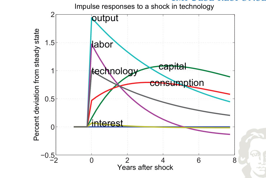
The path traces deviations after the initial disturbance, holding later innovations at zero. The shape results from current factor decisions, persistent productivity and the capital accumulated in previous periods; the response should be interpreted as an equilibrium deviation rather than a forecast of calendar-date data.
Fit to text
Scroll horizontally to inspect the labels and values.
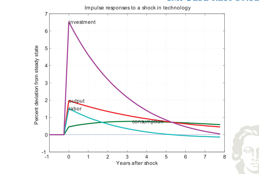
Impulse responses to a shock in technology
Fit to text
Scroll horizontally to inspect the labels and values.
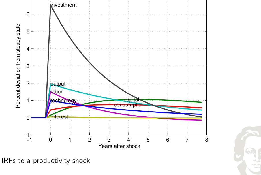
Economic propagation and quantitative assessment
A separate experiment introduces a one-percent deviation in inherited capital k₋₁, with productivity initially at steady state. Its response differs from the experiment that changes productivity at date zero.
Impulse Response
Fit to text
Scroll horizontally to inspect the labels and values.
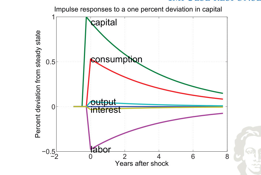
Fit to text
Scroll horizontally to inspect the labels and values.
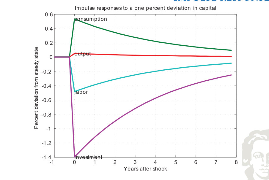
A Capital Stock Shock
A change in installed capital is propagated through different prices and incentives than a productivity innovation. Extra capital affects the marginal product of labor, the return on capital and the household’s future resources. The timing of capital availability is decisive: capital chosen as current investment is installed for subsequent production. The resulting transition highlights the importance of predetermined state variables.
Economic propagation and quantitative assessment
The model–data comparison evaluates relative standard deviations and cross-correlations, not merely the visual similarity of sample trajectories. It is important to apply compatible filtering rules to real and simulated series.
The quantitative comparison considers both dispersion and comovement. Relative standard deviations show that investment should fluctuate much more than output while consumption moves more smoothly; correlations summarize whether consumption, investment and hours are procyclical. A plausible sign pattern does not guarantee an exact empirical fit, and remaining deviations point toward mechanisms omitted from the benchmark.
Simulated Data
Fit to text
Scroll horizontally to inspect the labels and values.
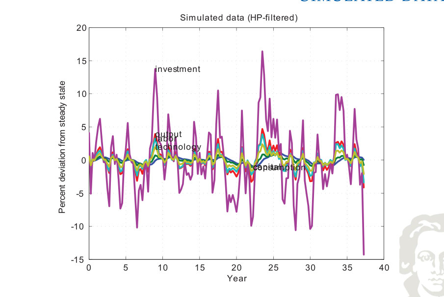
The simulated series are generated by a sequence of technology innovations and then HP-filtered. Their amplitudes and comovement provide model-implied business-cycle moments; unlike a single impulse response, many shocks contribute to the displayed path.
Synthesis
Impulse responses diagnose the propagation mechanism and simulations allow empirical comparison of RBC volatilities and comovements.
Appendix A. Notation and mathematical reference
This table consolidates notation used throughout the RBC framework. Time subscripts refer to the period; a bar indicates the deterministic steady state and a hat indicates the associated logarithmic deviation.
| Symbol | Meaning |
|---|---|
| Y, y | Gross domestic product / aggregate real output |
| C, c | Consumption |
| I, i | Gross investment |
| G | Government expenditures (in the introductory accounting model) |
| X, IM, Z | X denotes exports; IM or Z denotes imports in the national-accounts comparisons. In the Keynesian-cross diagrams, Z instead denotes planned aggregate expenditure; the local definition identifies the intended meaning. |
| kₜ₋₁ | Predetermined productive capital available in period t |
| nₜ, lₜ | Hours worked and leisure (nₜ + lₜ = 1) |
| zₜ | Stochastic productivity / total factor productivity in the RBC model |
| wₜ, rₜ | Real wage and competitive capital rental rate |
| πₜ | Firm profits distributed to the household |
| α, θ | Capital elasticity / capital factor-income share in Cobb–Douglas production |
| β | Household discount factor, 0 < β < 1 |
| δ | Capital depreciation rate |
| ϕ | Preference weight on leisure in the specialized utility function |
| ρ | Persistence of the log productivity process |
| uₜ | One-period technology innovation |
| Eₜ | Expectation conditional on information available at date t |
| σ, σᵤ | Standard deviation of technology innovations in the calibration; earlier σ is also used for utility curvature |
| x̄ | Steady-state level |
| x̂ₜ | Log deviation ln(xₜ/x̄) |
Important equilibrium equations
Production
A higher z raises output for given inputs; input elasticities sum to one.
Productivity dynamics
ρ summarizes propagation through the exogenous technology process.
Capital accumulation
Today’s installed investment makes capital available in the subsequent production period.
Wage schedule
Marginal product of labor equals the real wage.
Capital rental schedule
Marginal product of predetermined capital equals its rental price.
Time endowment
More labor reduces leisure, holding the endowment fixed.
Euler equation
The stochastic return enters tomorrow’s utility-weighted consumption opportunity.
Labor optimality
Under log consumption and linear leisure, work is chosen by equating its utility opportunity cost to its wage benefit.
Resource constraint
Closed-economy output is allocated between consumption and gross investment.
Steady-state capital return
The steady-state Euler condition determines the capital rental rate. The gross return on saving adds undepreciated capital: r̄ + 1 − δ = 1/β.
Steady-state investment
Replacement investment exactly offsets depreciation.
Log deviation
A log deviation is approximately a proportional difference when small; multiplying by 100 expresses it in percent.
Linearized production
A log-linear Cobb–Douglas identity is exactly additive in log variables.
Linearized labor equation
The linearized equilibrium condition after cancelling steady-state levels.
Linearized resource condition
Steady-state weights are necessary when adding deviations of different quantities.
Recursive solution
The policy rule separates responses to the two beginning-of-period states.
Equation consistency checks
- The household Euler equation uses the gross return rₜ₊₁ + 1 − δ, not the capital rental rate rₜ₊₁ alone.
- In period t, production uses kₜ₋₁ and not kₜ. Capital kₜ is selected by investment decisions at t and used in production at t+1.
- The coefficient on labor is 1−α in the no-growth Cobb–Douglas production function. Factor shares add to one under perfect competition and constant returns to scale.
- First-order log-linearization is a local percentage approximation. Never combine log-level equations with level resource weights without explicitly taking the approximation.
- Empirical business-cycle moments are estimates associated with a specific sample and data transformation, not universal constants that must hold for every country or period.
Appendix B. Review and self-study questions
These questions consolidate the core conceptual, mathematical and empirical ideas and provide a framework for independent study.
Models and microfoundations
1. Distinguish a quantitative equilibrium model from a purely accounting identity.
2. Explain endogenous versus exogenous variables in the basic RBC framework.
3. Why can an exogenous saving rule be unsuitable for a policy counterfactual?
4. Derive the simple Keynesian fiscal spending multiplier for fixed lump-sum taxes and explain the effect of proportional income taxation.
5. Discuss how leisure–consumption indifference curves relate to the marginal rate of substitution.
Empirical measurement
1. Distinguish trend growth, business cycles and seasonal movements.
2. Write the objective function of the Hodrick–Prescott filter and interpret its smoothing penalty.
3. State the five Kaldor balanced-growth facts and distinguish them from RBC cyclical facts.
4. Explain why output and investment should be measured in comparable real, seasonally adjusted units.
5. Interpret a relative standard deviation greater than one and a contemporaneous correlation near one.
Firm and shocks
1. Derive marginal products from Cobb–Douglas production and identify factor shares.
2. Explain why using kₜ instead of kₜ₋₁ changes the timing of the firm’s problem.
3. Compute the impulse path of an AR(1) process after a one-time innovation.
4. Explain why the Solow residual may reflect more than pure technological progress.
Household and equilibrium
1. Set up the representative household lifetime objective and period resource constraint.
2. Derive and interpret the Euler equation under log utility.
3. Derive the labor–leisure first-order condition for u(c,l)=ln(c)+ϕl.
4. Explain why consumption smoothing generates investment following a positive productivity disturbance.
5. Construct the five-equation RBC equilibrium system.
Steady state, calibration and solution
1. Find the steady-state return to capital in terms of β and δ.
2. Explain how the capital share and investment/output ratio are used in calibration.
3. Derive the log-linearized Cobb–Douglas production condition.
4. Why does the linearized resource constraint contain steady-state level weights?
5. Explain the role of stability and predetermined variables in the method of undetermined coefficients.
6. Interpret the P, Q, R and S matrices in a recursive toolkit solution.
Impulse responses and validation
1. Use the policy coefficients to calculate impact responses to a 1% productivity shock.
2. Describe how a shock affects investment and later capital through time.
3. Contrast a shock to current productivity with a deviation in installed capital.
4. Construct a simulation-based comparison using volatility and cross-correlation moments.
5. Identify two empirical features that the baseline RBC calibration fits imperfectly.
Further reading
The readings below develop the RBC framework and its extensions to monetary economics and nominal rigidities.
King, Robert G., and Sergio T. Rebelo (2000), “Resuscitating Real Business Cycles,” in Handbook of Macroeconomics, Vol. 1B.
George McCandless (2008), The ABCs of RBCs, Chapter 6.
Carl E. Walsh (2017), Monetary Theory and Policy, MIT Press, Chapters 7–8.
Jordi Galí (2015), Monetary Policy, Inflation, and the Business Cycle, Chapters 1–3.