
1. Microdata, evidence and causal questions
Econometric analysis turns observations about people, households, firms and other individual units into evidence about economic relationships. Its central challenge is not merely to calculate a correlation or fit a line. It is to establish what a comparison means, which explanation it supports and which alternative explanations remain possible. A large dataset can describe the world in great detail while still providing a misleading answer to a causal question.
What microdata reveal
Microdata record information at the level of individual observational units. A household survey may describe income, education, employment and insurance coverage; a firm dataset may report output, investment and employment; a school dataset may link student performance to resources and local characteristics. The prefix “micro” identifies the level of observation, not the size of the dataset. Millions of individual records are still microdata, whereas a short series of national output figures describes an aggregate.
The unit of observation must match the question. A relationship between average income and health across regions does not necessarily describe the relationship between individual income and individual health within each region. Aggregation changes both the comparison and the information available. Likewise, a school-district average cannot reveal every difference between students within a district. Before estimating a model, identify what each row represents, how observations enter the dataset and which population the observations are intended to represent.
Governments use these data to assess policies, businesses to understand demand, and non-profit organisations to evaluate interventions. Each application requires a decision about the relevant outcome. A programme may increase participation without improving final outcomes, or improve an average while leaving important groups worse off. Carefully defined variables and comparisons are therefore part of the substance of an analysis.
Data availability and data quality
Access to data does not guarantee reliable evidence. Errors may arise because a variable is recorded incorrectly, the sample excludes relevant people, definitions change over time or records are joined using imperfect identifiers. Missing income, for example, is not equivalent to zero income. If people with unusually high incomes are more likely to leave that question unanswered, deleting incomplete observations can change the population represented by the analysis.
Measurement deserves particular attention because many concepts are represented by imperfect proxies. A test score measures performance on a particular assessment, not every dimension of learning. An insurance indicator records coverage, not the quality or accessibility of care. A useful analysis explains the relationship between the concept of interest and the available measure, checks the coding and units, and considers how measurement limitations might affect the conclusions.
Data quality also includes the history of collection. Administrative records, surveys and experimental data are produced for different purposes and have different strengths. Administrative data may offer broad coverage but omit variables required for a causal comparison. A detailed survey may measure those variables but suffer from nonresponse. More observations improve precision under suitable conditions; they do not automatically correct an unrepresentative sample or a misleading definition.
Correlation and causation
Two variables are correlated when they vary together statistically. Causation asks whether changing one variable would change the other. The distinction is essential because a correlation can arise through several mechanisms: one variable may affect the other, the direction of influence may run in reverse, a third factor may affect both, or the relationship may occur by chance.
A deliberately striking example pairs US spending on science, space and technology with deaths by hanging, strangulation and suffocation over 1999–2009. The two series move together in the displayed period, but this does not establish that changing science spending changes those deaths. Trending series can appear closely related even when no credible causal mechanism connects them. Selecting an interesting pair after searching many series makes such coincidences especially easy to find.
More plausible relationships need the same scrutiny. Insured people may be healthier than uninsured people because insurance improves access to care. They may also differ in income, education, employment and initial health. A comparison of observed health combines these possibilities. To isolate an insurance effect, the analysis needs a reason to believe that the comparison represents what would happen to otherwise comparable people under different insurance conditions.
A causal claim therefore contains a counterfactual: what would have happened without the change being studied? The counterfactual is usually unobserved. Research design specifies how other observations can provide a credible substitute for it.
Description, prediction and intervention
Descriptive analysis characterises observed data: means, distributions, differences between groups and changes over time. Predictive analysis asks how well available information forecasts an outcome in observations that were not used to fit the model. Causal analysis asks how an intervention changes an outcome. These are different objectives, even when they use similar statistical tools.
A historical example illustrates the distinction. A 2012 report described the travel platform Orbitz as presenting more expensive hotel options to Mac users after finding that they tended to spend more on accommodation than Windows users. Device type could be useful for predicting spending because it is associated with customer characteristics. That association does not show that buying a Mac would itself increase a person's willingness to pay for a hotel. Nor does the reported ranking practice, by itself, demonstrate that identical rooms were sold at different prices.
Prediction can be valuable without a causal interpretation. Conversely, a model with excellent predictive accuracy may be unsuitable for evaluating a policy that changes the relationships on which the predictions depend. Econometric work should state its objective explicitly and judge the model against that objective. Machine-learning methods can support measurement, prediction and parts of causal estimation, but a flexible algorithm does not supply the missing identification argument.
Research design and the credibility of evidence
The emphasis on credible research design arose partly from concern that empirical conclusions could change with small alterations to specifications, assumptions or functional forms. Better computing and richer data made more elaborate analyses possible, but also made it easier to search across many models. The important response was to focus on why the variation used in an analysis can answer the causal question.
Random assignment provides a particularly clear benchmark because assignment is independent of potential outcomes. When experiments are infeasible, observational methods seek comparisons whose identifying assumptions can be stated and examined. Regression compares observations after accounting for measured characteristics. Panel methods use repeated observations of the same units. Difference-in-differences compares changes across groups under an assumption about their counterfactual trends. Each method succeeds only when its assumptions are appropriate to the setting.
Randomised evaluations of antipoverty programmes illustrate the connection between evidence and policy. The J-PAL research network uses such evaluations to study interventions and help decision-makers interpret the resulting evidence. The substantive lesson is that a programme's appeal or popularity is different from evidence about its effects. Evaluation asks what changes because of the programme and how that conclusion depends on the population, implementation and comparison being studied.
This shift is often called the credibility revolution in empirical economics. It does not imply that every recent empirical result is robust or causal. A persuasive analysis still requires transparent definitions, a defensible comparison, an appropriate treatment of uncertainty and checks targeted at plausible alternative explanations. A sophisticated estimator cannot compensate for a comparison that does not address the question.
From a question to a reproducible analysis
A sound empirical workflow begins with a precisely stated question and a definition of the population, treatment, outcome and period. The next step is to inspect the data before fitting a model. Check whether identifiers are unique, whether numerical values have plausible units and ranges, and whether missing values or sample restrictions change the composition of the data. Describe the outcome distribution and inspect the main relationships graphically.
Model selection then follows the research question and design. An estimate should be reported with its units, the relevant comparison and an assessment of uncertainty. For instance, a coefficient measured in test-score points per additional student per teacher answers a different question from a percentage change in test scores. Interpretation also requires distinguishing statistical precision from practical importance: a precisely estimated change can be small in substantive terms.
Reproducibility means keeping the transformations from raw observations to final results explicit. Stata, R and Python can all implement this workflow. The essential features are documented cleaning decisions, code that can be rerun, clear sample definitions and tables or figures that agree with the underlying calculations. Sensitivity checks should address specific concerns, such as omitted characteristics, unusual observations or alternative measurement choices.
Economic and political applications
Microeconometric methods can address questions far beyond a narrow definition of market behaviour. Examples include whether insurance improves health, whether smaller classes improve learning, whether legalising undocumented migrants affects mobility or political representation, and whether terrorist attacks alter electoral support. These questions combine individual or local data with mechanisms that are economically and socially important.
The same discipline applies across applications: define the change of interest, identify a comparison that can approximate its counterfactual, examine threats to that comparison and communicate the limits of the evidence. An estimated average effect describes a particular population and setting. Applying it elsewhere requires considering differences in institutions, behaviour and implementation. The following chapters develop the statistical tools needed to make these arguments explicit, beginning with randomisation and linear regression.
2. Randomisation and linear regression
A causal comparison should isolate the change of interest while holding relevant alternatives constant. Random assignment supplies a benchmark for this task. Linear regression provides a way to describe relationships and, under additional assumptions, to make comparable comparisons using observational data. Understanding the distinction between what an estimator calculates and what its identifying assumptions justify is essential to both approaches.
Health insurance and the problem of comparability
Consider whether health insurance improves health. Comparing insured and uninsured people appears straightforward: calculate average health in each group and subtract. The difficulty is that insurance coverage is not generally assigned at random. People with different coverage can also differ in income, education, employment, age and initial health. These factors may influence both coverage and subsequent outcomes.
The 2009 National Health Interview Survey illustrates the problem. Among married respondents in the reported sample, insured husbands had an average health index of 4.01, compared with 3.70 for uninsured husbands. The reported difference was 0.31. Insured wives also had a higher average index. Yet insured respondents were substantially more educated and had much higher family incomes. The comparison therefore combines insurance with other differences that might matter for health.
| Characteristic | Insured husbands | Uninsured husbands | Difference, husbands | Insured wives | Uninsured wives | Difference, wives |
|---|---|---|---|---|---|---|
| Health index | 4.01 [0.93] | 3.70 [1.01] | 0.31 (0.03) | 4.02 [0.92] | 3.62 [1.01] | 0.39 (0.04) |
| Nonwhite share | 0.16 | 0.17 | −0.01 (0.01) | 0.15 | 0.17 | −0.02 (0.01) |
| Age, years | 43.98 | 41.26 | 2.71 (0.29) | 42.24 | 39.62 | 2.62 (0.30) |
| Education, years | 14.31 | 11.56 | 2.74 (0.10) | 14.44 | 11.80 | 2.64 (0.11) |
| Family size | 3.50 | 3.98 | −0.47 (0.05) | 3.49 | 3.93 | −0.43 (0.05) |
| Employed share | 0.92 | 0.85 | 0.07 (0.01) | 0.77 | 0.56 | 0.21 (0.02) |
| Family income, US dollars | 106,467 | 45,656 | 60,810 (1,355) | 106,212 | 46,385 | 59,828 (1,406) |
The insured and uninsured samples contain 8,114 and 1,281 husbands, respectively, and 8,264 and 1,131 wives. Square brackets report standard deviations of the health index; parentheses report standard errors of differences. Differences are the originally reported estimates and can differ slightly from subtraction of the displayed rounded means. A standard deviation describes dispersion among individuals; a standard error describes uncertainty in an estimated mean or difference. Neither resolves the comparability problem.
Potential outcomes and selection bias
Let indicate insurance and its absence. Individual has two potential outcomes: is health with insurance and is health without it. The individual causal effect is . Only one potential outcome is observed for each individual at the relevant time:
The unobserved outcome is the counterfactual. The following hypothetical example makes the resulting problem concrete. Khuzdar chooses insurance and Maria does not. The observed comparison is , even though insurance improves Khuzdar's health by one point and has no effect on Maria's health.
| Quantity | Khuzdar | Maria |
|---|---|---|
| Health without insurance, | 3 | 5 |
| Health with insurance, | 4 | 5 |
| Chosen insurance status, | 1 | 0 |
| Observed health, | 4 | 5 |
| Individual causal effect | 1 | 0 |
Adding and subtracting Khuzdar's uninsured potential outcome decomposes the observed difference into the insurance effect and a pre-existing difference:
The general decomposition makes the target of the causal term explicit:
The first term is the average treatment effect on the treated, or ATT. The second is selection bias: the difference in untreated potential outcomes between the groups. It need not equal a difference that can be observed directly. Education and income may reveal some sources of selection; preferences, initial conditions or other unmeasured factors may reveal none. Nor is the ATT necessarily the average treatment effect for the whole population when effects differ across individuals.
Random assignment and the law of large numbers
Random assignment makes treatment status independent of potential outcomes. With a well-defined treatment and no interference between individuals, it implies that average untreated potential outcomes are equal across assignment groups in the population. It also makes treated and untreated groups comparable in their average treatment effects. The difference in group means can then identify the average causal effect.
Randomisation balances characteristics in expectation; it does not make every realised sample identical. A coin flip assigning one of two people to treatment plainly cannot ensure matching ages, incomes or genders. Larger samples tend to reduce accidental imbalances, but a large sample is not a substitute for genuinely random assignment. Random sampling and random assignment are also distinct: the former concerns representation of a population, while the latter concerns comparability of treatment groups.
The law of large numbers explains why averages stabilise. For independent, identically distributed observations with a finite expected value, a standard version states:
Convergence in probability means that the probability of a discrepancy larger than any fixed positive tolerance tends to zero as the sample grows. For a fair six-sided die, the expected result is . A running average can fluctuate widely at first and then settle near 3.5. It need not approach 3.5 monotonically, and no universal threshold such as 100 observations guarantees adequate precision.
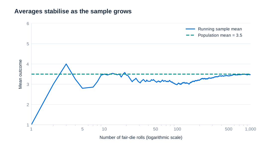
Sample-size requirements depend on outcome variability, the treatment effect of interest, the assignment scheme and the desired precision. Clustering can reduce the information provided by a nominally large sample because observations within a group may be correlated. Noncompliance, attrition and spillovers can also change the interpretation of an experiment. An effect of assignment to insurance, for example, need not equal the effect of actually receiving insurance if some people do not follow their assignment.
Reading a balance table
A balance table compares characteristics measured before treatment. It helps assess whether assignment groups look comparable and whether implementation or sample attrition has created concerning differences. The RAND Health Insurance Experiment provides an example comparing more generous plans with a catastrophic-coverage plan. The first numerical column below reports the catastrophic group's baseline mean. The other columns report differences from that mean, rather than the alternative groups' means themselves.
| Characteristic | Catastrophic mean | Deductible difference | Coinsurance difference | Free-care difference | Pooled alternative plans difference |
|---|---|---|---|---|---|
| Female share | 0.560 | −0.023 (0.016) | −0.025 (0.015) | −0.038 (0.015) | −0.030 (0.013) |
| Nonwhite share | 0.172 | −0.019 (0.027) | −0.027 (0.025) | −0.028 (0.025) | −0.025 (0.022) |
| Age, years | 32.4 [12.9] | 0.56 (0.68) | 0.97 (0.65) | 0.43 (0.61) | 0.64 (0.54) |
| Education, years | 12.1 [2.9] | −0.16 (0.19) | −0.06 (0.19) | −0.26 (0.18) | −0.17 (0.16) |
| Family income, US dollars | 31,603 [18,148] | −2,104 (1,384) | 970 (1,389) | −976 (1,345) | −654 (1,181) |
| Hospitalised in the previous year, share | 0.115 | 0.004 (0.016) | −0.002 (0.015) | 0.001 (0.015) | 0.001 (0.013) |
| General health index | 70.9 [14.9] | −1.44 (0.95) | 0.21 (0.92) | −1.31 (0.87) | −0.93 (0.77) |
| Cholesterol, mg/dl | 207 [40] | −1.42 (2.99) | −1.93 (2.76) | −5.25 (2.70) | −3.19 (2.29) |
| Systolic blood pressure, mm Hg | 122 [17] | 2.32 (1.15) | 0.91 (1.08) | 1.12 (1.01) | 1.39 (0.90) |
| Mental health index | 73.8 [14.3] | −0.12 (0.82) | 1.19 (0.81) | 0.89 (0.77) | 0.71 (0.68) |
Standard deviations, where reported for the catastrophic group, appear in brackets; standard errors of differences appear in parentheses. Enrolment was 759 in catastrophic coverage, 881 in the deductible plan, 1,022 in coinsurance and 1,295 in free care. The last column pools the 3,198 participants in the three alternative plans. Catastrophic coverage is itself insurance, so this is a comparison of insurance generosity, not a comparison with complete absence of coverage.
For example, the free-care group's female share is approximately . Its baseline general health index is approximately . The table does not show the effect of free care on health: these are baseline characteristics, measured before treatment could produce the subsequent outcomes of interest.
Some baseline differences can be statistically significant by chance, especially when many characteristics are examined. The free-care difference in the female share is about 2.53 standard errors from zero. That observation should be interpreted with the assignment procedure and the full pattern of balance, rather than treated as automatic proof that randomisation failed. Conversely, insignificant differences do not prove that unobserved characteristics are balanced or that there is no important imbalance in a small sample.
The population model and the least-squares solution
When random assignment is unavailable, a regression can describe how an outcome varies with an explanatory variable. The simple linear model is:
Here is the outcome, the explanatory variable, the intercept and the slope. The disturbance collects the outcome's remaining determinants and deviations from the specified relationship. The coefficients are population quantities; their estimates vary across samples. The disturbance is an unobserved random variable, not a fixed population parameter.
Ordinary least squares, or OLS, chooses the intercept and slope that minimise the sum of squared vertical deviations between observed outcomes and the fitted line:
Squaring prevents positive and negative deviations from cancelling and puts greater weight on large discrepancies. Differentiating with respect to the two coefficients gives the normal equations and . Solving them, when varies in the sample, yields:
The denominator is a sum of squared deviations. Without the square, the deviations around the sample mean sum to zero. The slope can equivalently be written as the ratio of sample covariance to sample variance, provided both use the same normalisation. Under the appropriate population orthogonality condition, the corresponding population slope is .
Fitted values, residuals and regression geometry
The fitted value is . The residual is the observed outcome minus this prediction, . It is a vertical distance because the criterion predicts conditional on ; OLS does not minimise perpendicular distances to the line.
In one numerical illustration, the fitted line is and the sum of squared residuals is 384. At , the line predicts 23.07. An observation above that value has a positive residual and one below it a negative residual. The value 384 describes total squared discrepancies in the sample and depends on the outcome's scale and the number of observations; it is not by itself a measure of causal credibility.
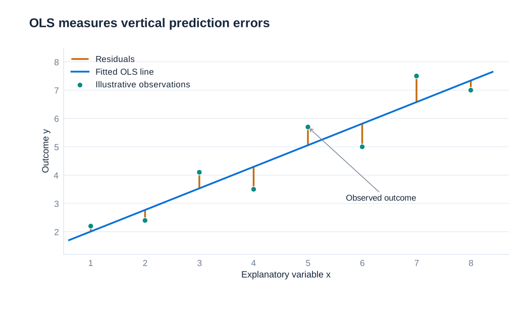
With an intercept, the normal equations imply exact sample identities:
The line therefore passes through , and residuals are orthogonal to the included regressor and fitted values in the sample. These are algebraic properties of the OLS calculation. They do not establish that the population disturbance is unrelated to . An omitted determinant correlated with can bias the coefficient even though the fitted residuals satisfy every one of these identities.
Keeping and distinct prevents a common error. The former belongs to the population model and is not directly observed; the latter is calculated after estimating the model. Inspecting residuals can reveal patterns, unusual observations or inappropriate functional forms, but zero sample covariance between an included regressor and its OLS residuals is guaranteed by construction.
Test scores and the meaning of a slope
A dataset of 420 California school districts relates average test scores to the student-to-teacher ratio. The fitted relationship, using the reported coefficient estimates rounded to two decimal places, is:
The slope associates one additional student per teacher with a 2.28-point lower predicted test score. A reduction in the ratio by two students per teacher corresponds to a 4.56-point increase in the fitted outcome. At a ratio of 20, the prediction is ; at a ratio of 18 it is 657.86. These are predictions from the estimated line, not the observed outcome of every district with those ratios.
Relative to a mean test score of approximately 654, a 2.28-point change is about . This calculation gives scale to the coefficient. It does not make 0.35% the regression coefficient, and it is not a 0.35-percentage-point change. In a linear-linear model, the direct coefficient always measures outcome units per explanatory-variable unit.
The intercept is the predicted outcome when the student-to-teacher ratio is zero, which lies outside the relevant data range. It helps position the fitted line but has little substantive value as a literal prediction. Extrapolating far beyond the observed range is risky because a linear pattern within that range need not continue elsewhere.
Most importantly, the negative slope alone does not show that hiring teachers causes the predicted improvement. District income, language composition and other resources may be associated with both class size and test scores. Regression adjustment can compare districts with similar measured characteristics, but controlling for observables does not automatically eliminate unobserved differences. A causal interpretation requires an argument about the determinants left in the disturbance.
Unbiasedness, consistency and the bias–variance trade-off
An estimator is a rule applied to a sample; an estimate is its realised numerical result. Repeating the sampling process produces a sampling distribution. Unbiasedness means that the average of this distribution equals the population parameter: . It does not mean that every estimate equals the parameter. An unbiased estimator can be imprecise and produce individual estimates far from the truth.
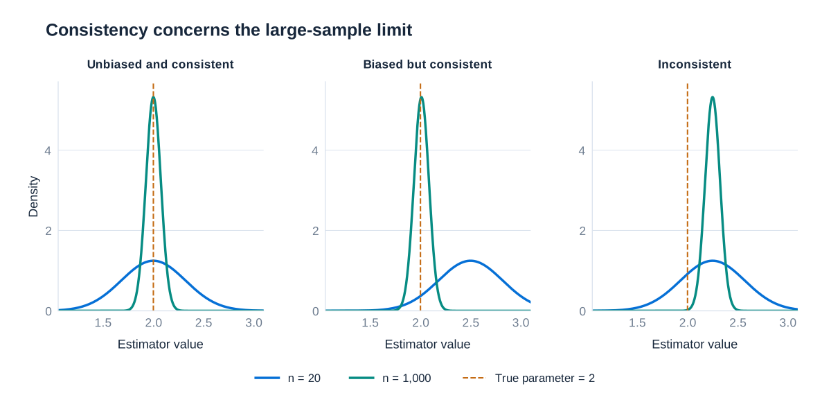
Consistency concerns a sequence of estimators as sample size increases. Formally, . The probability of a fixed-size estimation error then tends to zero. Unlike unbiasedness, consistency is an asymptotic property. More observations do not make an inherently inconsistent procedure consistent; they can instead concentrate its estimates around the wrong value.
Three examples distinguish these concepts. First, suppose satisfies the conditions for unbiased and consistent OLS. The slope distribution is centred on 2 and becomes more concentrated as the sample grows. Second, define a modified estimator . It has finite-sample bias but is consistent when OLS is consistent: the added term is 0.5 at , 0.01 at , and tends to zero.
Third, suppose the disturbance in the same structural equation is , with . Substitution gives . A regression of on converges to 2.25, not the structural coefficient 2. Increasing sample size makes the descriptive slope more precise while leaving the 0.25 discrepancy in the structural interpretation.
Precision and bias are separate dimensions of performance. For a scalar estimator, mean squared error decomposes as:
An estimator with a small bias may have lower mean squared error than a very dispersed unbiased estimator. This trade-off matters when evaluating estimators, but it does not justify ignoring systematic causal bias merely because standard errors are small.
The assumptions behind OLS properties
For the familiar finite-sample unbiasedness result, a central condition is zero conditional mean, , together with a correctly specified linear conditional mean, suitable sampling conditions and variation in . Zero unconditional mean, , is weaker: positive and negative errors can average to zero while still varying systematically with the regressor. Zero covariance between and can support consistency of a linear projection under appropriate regularity conditions, but it should not be presented as equivalent to zero conditional mean.
In multiple regression, the regressors must not be perfectly collinear. In the simple model this means that cannot be constant. Without variation in , the data cannot distinguish the intercept from the slope. Random sampling and finite-moment conditions support laws of large numbers and sampling approximations. Very influential observations require investigation; the formal requirement is not that no unusual observation may exist.
The Gauss–Markov result adds homoskedasticity and absence of correlation between disturbances across observations, conditional on the regressors. Under the relevant assumptions, OLS is the best linear unbiased estimator, or BLUE. “Best” means smallest variance within the class of linear unbiased estimators. “Linear” refers to the estimator being a linear function of observed outcomes, conditional on the regressors. It does not mean that only straight-line relationships can be modelled, nor does it mean that OLS dominates every possible nonlinear or biased estimator.
Normal disturbances are not required for Gauss–Markov. Heteroskedasticity can leave OLS unbiased and consistent under exogeneity while invalidating the usual homoskedastic variance formula and the BLUE claim. Finally, even correct estimation of a conditional association does not automatically establish a causal mechanism: the economic interpretation depends on the research design and the meaning of the disturbance.
What determines precision?
Under homoskedasticity and uncorrelated disturbances, the conditional variance of the simple-regression slope is:
The exact expression conditions on the realised regressor values; the approximation replaces their sum of squared deviations with its large-sample counterpart. Greater disturbance variance makes the line harder to estimate. Greater variation in provides more information about its slope. More observations generally improve precision when they add independent information. The standard error, being the square root of variance, typically decreases at a rate proportional to , so quadrupling sample size approximately halves it under otherwise comparable conditions.
In practice the unknown disturbance variance must be estimated. With an intercept and one slope, a conventional homoskedastic estimator is , giving . The subtraction of two reflects the two estimated coefficients. Heteroskedasticity or dependence requires a variance estimator appropriate to that setting.
Reading a regression result therefore involves three distinct questions. What comparison and units does the coefficient represent? Which assumptions justify interpreting it as the target relationship? How much sampling uncertainty remains? Answering only the first or third can produce an apparently precise conclusion that the design does not support.
3. Omitted Variable Bias and Measurement Error
A regression coefficient is useful only when its interpretation matches the process that produced the data. A large sample can make an estimate very precise while leaving it systematically wrong about the relationship of interest. Two particularly important threats are omitted variables, which place relevant determinants of the outcome inside the regression error, and measurement error, which separates the variables recorded in a dataset from the economic quantities they are supposed to represent. Understanding these problems requires distinguishing uncertainty around an estimate from bias in its target.
Consistency, exogeneity, and the target of estimation
Consider the population relationship . The parameter describes the relationship we seek to estimate; the error collects determinants of the outcome that are outside the model. In a simple regression with an intercept, the OLS slope can be expressed as a sample covariance divided by a sample variance. Under a law of large numbers and a positive, finite variance of , its probability limit is
The equation identifies the central consistency requirement: the regressor must be uncorrelated with the error for OLS to converge to this structural slope. The stronger condition also supports the usual conditional interpretation and, with suitable sampling assumptions, finite-sample unbiasedness. Consistency means that the estimator approaches the target as the sample grows; unbiasedness concerns the estimator's expectation at a particular sample size. Neither property is established simply by obtaining a small standard error.
The statement that OLS is the best linear unbiased estimator additionally requires the assumptions of the Gauss–Markov theorem, including the appropriate homoskedastic and uncorrelated error structure. Those efficiency assumptions should not be confused with the exogeneity conditions needed to recover the target coefficient. A regression can have heteroskedastic errors and still estimate the slope consistently, whereas an omitted confounder can make the coefficient inconsistent even with perfectly homoskedastic errors. If the goal is only a best linear prediction, OLS can estimate that predictive projection without identifying a causal effect.
Deriving omitted variable bias
Suppose that the relevant population model contains an additional variable :
where is uncorrelated with and . If is omitted, the error in the shorter regression becomes . The omission matters for the coefficient on when two conditions hold together: helps determine , so that , and is correlated with . Correlation with alone is insufficient if the omitted variable has no effect on the outcome in the relevant population relationship.
Write the population linear projection of the omitted variable on the included regressor as
This projection is an algebraic description of association; it does not require to cause . Substitution gives
The short-regression slope therefore converges to a combination of the direct slope and the association operating through the omitted variable:
This is a statement about the probability limit, not an exact decomposition of every realized estimate: an individual sample also contains sampling variation. In multiple regression, the corresponding omitted-variable relationship is conditional on the controls already included. What matters is whether the omitted variable remains related to the regressor after those controls have been taken into account.
Determining the direction of the bias
The sign of the bias is the product of two signs. First ask whether an increase in the omitted variable raises or lowers the outcome, holding the included regressor fixed. Then ask whether observations with larger values of the included regressor tend to have larger or smaller values of the omitted variable. Keeping these two questions separate prevents an intuitive story from being substituted for an actual sign calculation.
| Effect of omitted variable on the outcome | Association with the included regressor | Bias in the short-regression slope |
|---|---|---|
| Positive: | Positive: | Positive: slope is shifted upward |
| Positive: | Negative: | Negative: slope is shifted downward |
| Negative: | Positive: | Negative: slope is shifted downward |
| Negative: | Negative: | Positive: slope is shifted upward |
“Upward” means numerically larger, and “downward” means numerically smaller. Neither expression is synonymous with “closer to zero.” A negative bias makes a positive coefficient smaller, but makes a negative coefficient more negative; sufficiently strong confounding can even reverse its sign. When several relevant variables are omitted, their contributions can reinforce or offset one another, so identifying one plausible confounder need not identify the sign of the total bias.
Test scores, class size, and family income
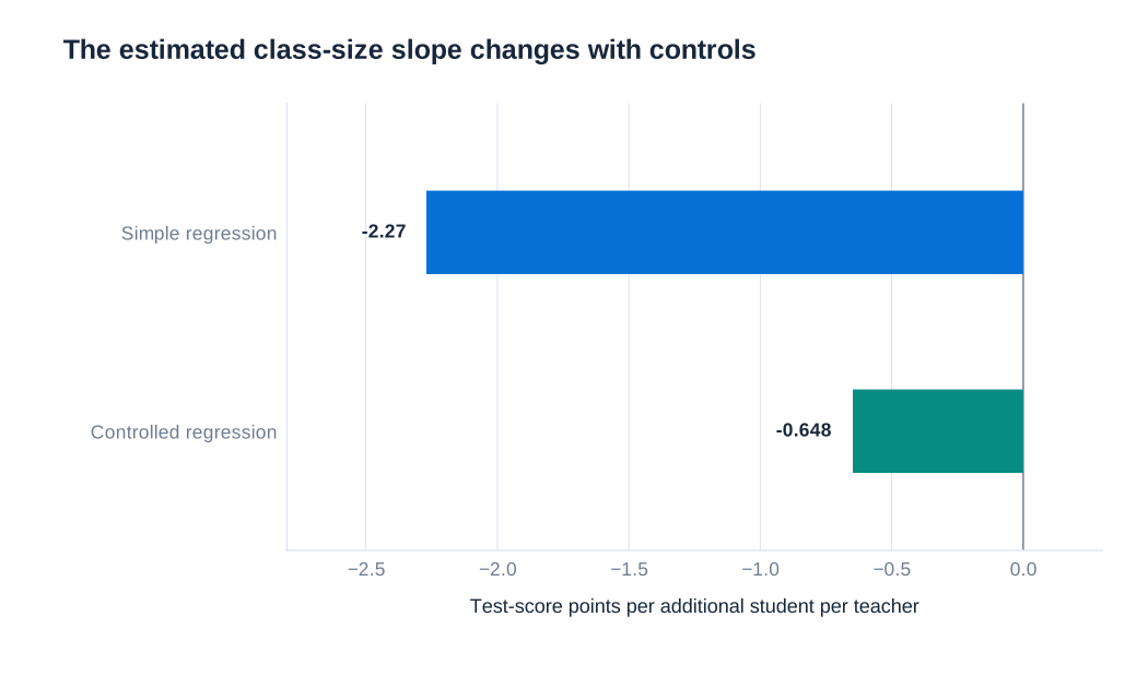
A school-district example relates average test scores to the student-to-teacher ratio. A higher ratio means more students per teacher, so the coefficient is measured in test-score points per additional student per teacher. The unadjusted regression gives an intercept of approximately and a slope of approximately . It predicts that districts differing by one student per teacher differ by about 2.28 test-score points on average. This is initially an association between districts, not an identified effect of hiring teachers.
Family income offers a plausible explanation for part of that association. Suppose that higher family income raises achievement through resources and opportunities, so , and that richer districts tend to have lower student-to-teacher ratios, so . Their product is negative. The short regression then attributes some of the achievement advantage associated with income to the lower ratio, making the estimated ratio coefficient more negative than the coefficient obtained with a suitable income control.
In the illustrated comparison, the displayed ratio slope changes from approximately without income to with income. A five-unit increase in the ratio is consequently associated with about points using the first displayed slope and points using the adjusted slope. These are calculations from the reported regression slopes, not experimental policy effects. The upward movement of the coefficient is consistent with the predicted direction of omitted income bias, but does not establish that all confounding has disappeared.
The adjustment should be understood as comparing districts after accounting for the modeled income relationship. Other determinants, including family background, school composition, and the way resources are allocated, may remain relevant. A fitted intercept near 699 is also an extrapolation to a ratio of zero, outside the useful comparison range; it should not be interpreted as the score a real district would obtain with no students per teacher.
Addressing omitted variables without adding bad controls
The most direct response is to collect and include a well-measured confounder. This works only if the expanded model provides an adequate representation of the relevant conditional relationship and sufficient variation remains to estimate the effect. Controlling for a variable does not automatically remove every dimension of selection associated with it. For example, one income measure may leave substantial differences in family resources unexplained, and a purely linear adjustment may be inadequate for a strongly nonlinear relationship.
A proxy can help when the confounder itself is unavailable, but an imperfect proxy generally leaves residual confounding. Instrumental variables can address certain endogeneity problems when an instrument is relevant for the endogenous regressor and satisfies a credible exclusion restriction and exogeneity condition. Panel methods can remove unobserved characteristics that remain constant within a unit over time. Each approach replaces one identification challenge with explicit assumptions that must be defended; none is a mechanical guarantee of a causal coefficient.
Control selection should follow the causal question. A variable caused by the treatment can be a mediator rather than a pre-existing confounder. Adjusting for it may remove part of the total effect that the researcher wants to estimate. Conditioning on a common consequence of treatment and unobserved outcome determinants can also create bias. A thoughtful specification therefore begins with a description of the economic process and the timing of variables, rather than with a search for the largest possible collection of controls.
Measurement error in an explanatory variable
Economic variables are frequently measured imperfectly. National output relies on incomplete records and estimation; time-use surveys depend on recall; undocumented migration is difficult to count; self-reported income and happiness may be recorded inaccurately. Measurement error can reflect random noise, systematic reporting behavior, or a mismatch between a recorded indicator and the underlying concept.
Let denote the true regressor and let the observed value be . Suppose the population model is . In the classical additive case, assume , , , and . Substituting into the model yields
The minus sign is essential. The observed regressor contains the measurement error positively, while the new regression disturbance contains it multiplied by . Consequently,
Thus even error that is unrelated to the true regressor creates correlation between the observed regressor and the composite regression disturbance. Calling the measurement error “random” does not make the resulting regression exogenous.
Attenuation, reliability, and nonclassical error
The classical assumptions imply and . The probability limit of the observed-regressor slope is therefore
The reliability ratio lies between zero and one when true variation is positive and measurement-error variance is finite. It equals one when there is no measurement error. As noise becomes more important relative to true variation, the slope is pulled further toward zero. A positive true coefficient is attenuated downward; a negative true coefficient is attenuated upward. Attenuation is therefore a reduction in magnitude, not an invariably downward numerical bias.
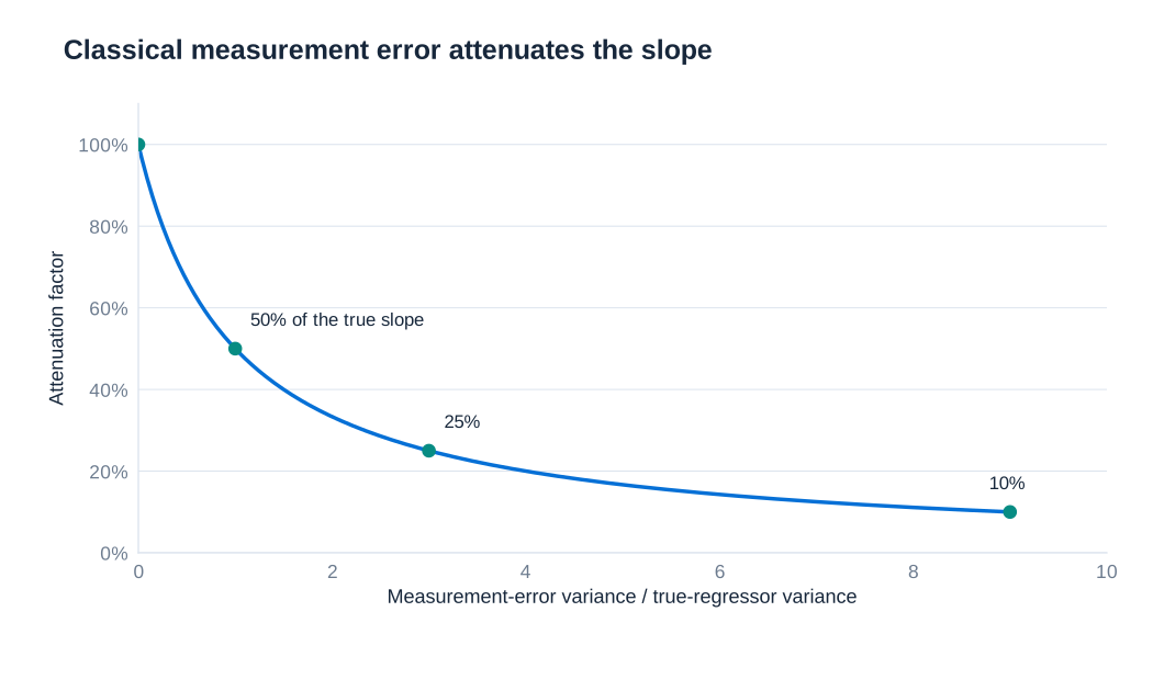
For a hypothetical example, if true variation and measurement-error variation are equal, then : a true slope of 4 is estimated near 2 in a sufficiently large sample, while a true slope of is estimated near . More observations concentrate the estimator around this attenuated target; they do not remove the distortion. Better measurement, validation information, or a suitably valid instrument can help identify the desired coefficient.
Nonclassical error violates one or more of the classical restrictions. High-income respondents might underreport income more strongly, or reporting quality might depend on the outcome. The bias can then have either sign. Even classical error in one variable of a multiple regression need not move every estimated coefficient toward zero: correlations among regressors can transmit the problem to other coefficients. The simple reliability formula should therefore be used only for the model and assumptions under which it was derived.
Measurement error in the outcome and practical interpretation
Now suppose the true outcome satisfies , but the observed outcome is . The estimated relationship becomes
If the original error is exogenous and the outcome measurement error has conditional mean zero given , the composite error remains exogenous. The slope can therefore remain consistent. If is also uncorrelated with , its variance adds to the original disturbance variance, generally reducing precision. Under those restrictions, classical outcome noise increases uncertainty without producing the regressor attenuation described above.
This conclusion is conditional, not universal. If people with higher systematically overreport the outcome, then varies with and the slope can be biased. Correlation between measurement error and the original disturbance also changes the simple variance-addition result. A careful empirical analysis identifies what is measured, how it is recorded, and why the proposed error assumptions are plausible. The central distinction is whether the problem changes the coefficient's target, its precision, or both.
4. Hypothesis Testing and Statistical Inference
A point estimate is one realization of a procedure applied to data. Another sample could produce another estimate, even if the population relationship remained unchanged. Statistical inference measures this sampling uncertainty and uses it to assess hypotheses and construct confidence intervals. Its conclusions depend both on a credible model for the coefficient and on a credible estimate of the coefficient's variability. Neither a small p-value nor a narrow interval repairs omitted variable bias or an invalid causal design.
Random sampling and random assignment answer different questions
Random sampling concerns how observations enter a dataset. A simple random sample supports inference from the observed units to the population from which they were drawn. Random assignment concerns how treatment is allocated among units and can make treatment status independent of their potential outcomes. A study can have random assignment without drawing a representative population sample, or a representative sample without random treatment assignment.
The distinction separates identification from generalization. Random assignment can provide a credible treatment comparison within the studied group; extending that effect to other groups may require additional assumptions. Conversely, randomly sampling people does not make their education, income, or treatment choices exogenous. In observational regression, uncertainty about which units were sampled and bias from how the regressor is related to unobserved determinants are different problems.
The sampling distribution describes the estimates that would arise if the sampling procedure were repeated under the same population and model. This is a conceptual repetition, not a claim that the researcher actually observes many populations. Standard errors approximate the spread of that distribution using the available data and assumptions about dependence. If the sampling process involves households, schools, regions, or repeated observations, the relevant independent units may be groups rather than individual rows.
Standard errors measure uncertainty in an estimator
The standard deviation of an outcome describes variation across observations. The standard error of an estimator describes variation across hypothetical repeated estimates. These quantities answer different questions and have different units. A regression slope's standard error is measured in the same units as that slope: for a test-score regression on students per teacher, it is test-score points per unit of the ratio.
For a simple regression with an intercept, conditionally homoskedastic and uncorrelated errors, and a valid conditional-mean specification, the slope variance conditional on the observed regressors is
Because the disturbance variance is unknown, it is estimated from residuals. With two estimated coefficients, the usual estimator is . The conventional slope standard error is the square root of the estimated coefficient variance. The corresponding large-sample intuition is .
More unexplained outcome variation increases uncertainty; more independent observations and more useful regressor variation reduce it. In multiple regression, the useful variation in a regressor is what remains after accounting for the other regressors. Strong collinearity can therefore produce large standard errors even in a dataset with many observations. These relationships concern precision under the model, not whether the model identifies a causal effect.
Null hypotheses, t-statistics, and reference distributions
A null hypothesis specifies a value for a population parameter, such as . For a two-sided alternative, , the t-statistic measures the estimated distance from the null in standard-error units:
When , this reduces to the familiar coefficient-to-standard-error ratio. A value of means that the estimate is four estimated standard errors below the hypothesized value. It is the population coefficient that the hypothesis concerns; the observed estimate is already known and is not itself a random unknown after the data have been observed.
Under normally distributed, conditionally homoskedastic independent errors and the usual linear model assumptions, the conventional t-statistic has an exact Student t distribution with degrees of freedom, where includes the intercept. With heteroskedasticity-robust standard errors, that exact finite-sample result generally does not apply. Under appropriate regularity conditions, the studentized statistic instead approaches a standard normal distribution as the effective sample size grows. Software may use a t reference distribution with a degrees-of-freedom adjustment as an approximation; its validity should be assessed in light of the design.
The central limit theorem applies to standardized averages
The central limit theorem explains why normal approximations can be useful even when individual observations are not normally distributed. For independent and identically distributed random variables with mean and finite positive variance , the basic theorem states
The raw observations do not become normal as the sample grows. The centered and scaled sample mean approaches a normal distribution, while the unscaled sample mean becomes concentrated near its population mean. Regression inference uses a related argument because, under suitable assumptions, an estimator's error can be represented approximately as an average of random contributions. Valid studentization additionally requires a consistent standard-error estimate.
Consider a Bernoulli variable that equals one with probability 0.8 and zero otherwise. Each observation remains binary for every sample size. Its mean is 0.8 and its variance is . The standard deviation of its sample mean is therefore . At sample sizes 10, 100, 1,000, and 10,000, this becomes approximately 0.1265, 0.0400, 0.01265, and 0.0040 respectively.
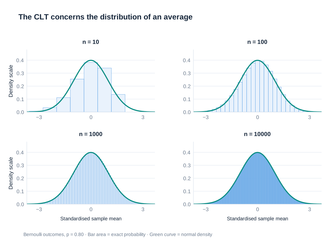
The distribution of the sample mean is discrete, with possible values separated by . At small sample sizes it can be visibly asymmetric because the success probability is high; at larger sizes its standardized shape is well approximated by the normal distribution. The approximation is not an automatic consequence of a large row count. Heavy tails, dependence, weak identification, or only a few independent clusters can undermine the conditions required for familiar large-sample reasoning.
Rejection regions and statistical significance
A significance level specifies the probability of rejecting a true null hypothesis that the testing procedure is designed to control under its assumptions. For a two-sided test using a standard normal reference distribution, a 5% significance level places 2.5% in each tail and uses critical values approximately and . Rejecting when therefore identifies estimates unusually far from the null relative to their estimated sampling variability.
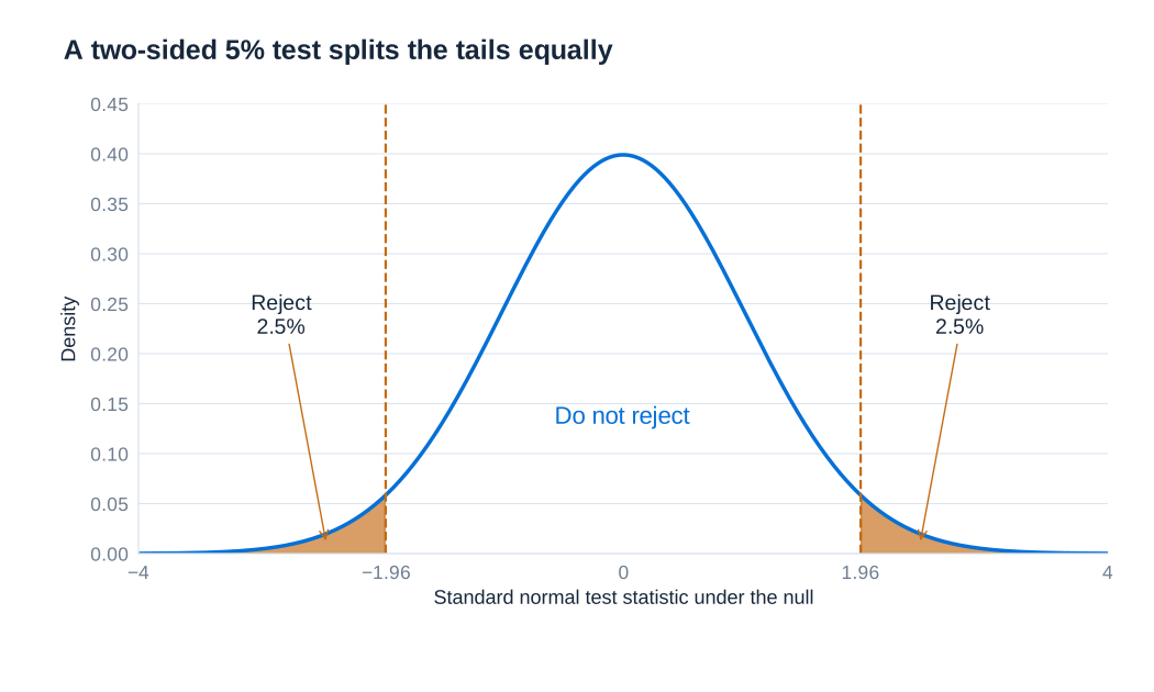
The familiar statement that about 95% of a normal distribution lies within two standard deviations is a useful approximation; the exact central normal probability between and is about 95%, whereas the interval from to contains about 95.45%. An exact t test uses a critical value based on its degrees of freedom, which is larger than 1.96 in finite samples.
A rejection does not establish a 95% probability that the alternative is true. A failure to reject does not establish that the null is true. Tests can make a Type I error by rejecting a true null or a Type II error by failing to reject a false null. Power is the probability of rejecting under a specified alternative; small samples and noisy measurements can make economically important effects difficult to detect. One-sided tests allocate their rejection region to one direction and should be justified before examining the estimated sign.
P-values express incompatibility with the null model
A p-value is the probability, calculated under the null hypothesis and the maintained statistical assumptions, of obtaining a test statistic at least as extreme as the observed one. For a two-sided standard normal test,
where is the standard normal cumulative distribution function. With an appropriate t reference distribution, its cumulative distribution replaces . The calculation includes outcomes more extreme than the observed statistic; it is not the probability of obtaining exactly that estimate.
A p-value of 0.04 means that, if the null and the statistical model held, a statistic at least as extreme would occur with probability 4%. It is evidence against that null at the 5% level, not a 4% probability that the null is true or proof that the estimated effect is causal. A p-value of 0.50 indicates weaker evidence against the null, but does not demonstrate that the true effect is zero. It may reflect a small effect, imprecise estimation, or both.
Statistical significance also differs from economic importance. A tiny effect can yield a small p-value in a very large sample, while a large but imprecise estimate may not cross a conventional threshold. The effect's units, confidence interval, substantive relevance, and identification assumptions should accompany the p-value. Testing many outcomes or specifications and reporting only the smallest p-values changes the interpretation of nominal significance levels.
Confidence intervals retain information about magnitude
A two-sided confidence interval combines the estimate with a margin of uncertainty:
where is the critical value corresponding to the confidence level and reference distribution. A 95% confidence procedure is constructed so that, over repeated samples under its assumptions, approximately 95% of the resulting intervals contain the fixed population parameter. Once a particular interval has been calculated, its endpoints are fixed and the parameter either lies inside it or does not; the frequentist interpretation is not a posterior probability assigned to that parameter.
When the interval and test use the same assumptions and reference distribution, the interval contains the null parameter values that the corresponding two-sided 5% test would not reject. If zero is outside a 95% interval, the coefficient is statistically distinguishable from zero at that level. If zero is inside, the interval may still include economically substantial positive or negative values. Reading the whole interval therefore gives more information than attaching a significance star to the point estimate.
A complete test-score regression example
The regression of district average test scores on the student-to-teacher ratio uses 420 observations and heteroskedasticity-robust standard errors. The estimated equation is . The regression explains about 5.12% of the sample outcome variation, so . Its root mean squared error is 18.581 test-score points. These fit statistics describe the regression's sample fit and residual scale, not the validity of a causal interpretation.
| Regressor | Coefficient | Robust standard error | t-statistic | Two-sided p-value | 95% confidence interval |
|---|---|---|---|---|---|
| Student-to-teacher ratio | −2.279808 | 0.5194892 | −4.39 | < 0.001 | [−3.300945, −1.258671] |
| Intercept | 698.933 | 10.36436 | 67.44 | < 0.001 | [678.5602, 719.3057] |
Testing a zero ratio coefficient gives . The output uses 418 residual degrees of freedom and reports for the one-coefficient restriction; in this case the F-statistic is the squared t-statistic, up to rounding. The two-sided p-value for the ratio coefficient using this t reference is approximately 0.0000145. A displayed p-value rounded to 0.000 therefore means very small, not literally zero.
The 95% t critical value for 418 degrees of freedom is approximately 1.96566. Applying it gives the reported interval . The normal approximation using 1.96 gives the very similar interval . Mixing a heavily rounded coefficient, a different critical value, and more precise printed endpoints would create apparent arithmetic discrepancies, so calculations should retain the original precision until the final reporting step.
The interval describes uncertainty about the regression association under the maintained model. A one-unit higher ratio is associated with a decrease between about 1.26 and 3.30 test-score points at this confidence level. The omitted-income argument in the preceding chapter still applies: robust standard errors address a variance problem, not the confounding that can separate this coefficient from the causal effect of changing class size.
Heteroskedasticity and robust standard errors
Homoskedasticity means that the conditional disturbance variance is constant: . Heteroskedasticity means that this variance changes with the regressors or other observed characteristics. A graph may show observations spreading more widely around the conditional mean at larger values of . The slope of that mean and the width of the disturbance distribution are separate features of the model.
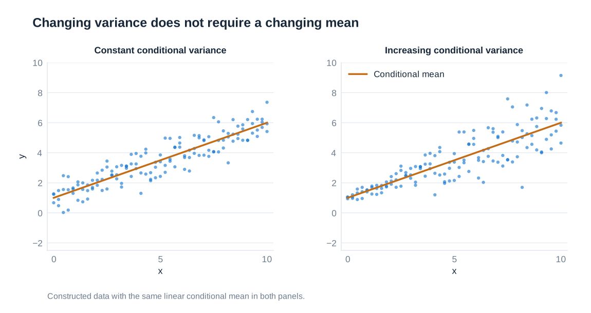
If exogeneity and the relevant sampling conditions continue to hold, heteroskedasticity does not by itself make OLS coefficients inconsistent. It does invalidate the conventional homoskedastic variance formula. Standard errors calculated from that formula can be too small or too large; downward distortion and overstated significance are common concerns, but the direction is not guaranteed.
For simple regression with an intercept and independent observations, the basic heteroskedasticity-robust variance estimator can be written
Each squared residual contributes separately, allowing the disturbance variance to differ across observations. Other robust estimators adjust for degrees of freedom or leverage; the HC1 version multiplies the variance estimate by . Changing from conventional to robust standard errors leaves the OLS point estimates unchanged when the regression sample and specification are unchanged, but can change confidence intervals, t-statistics, and p-values.
Heteroskedasticity-robust standard errors are not a general correction for dependence between observations, omitted variables, or measurement error. They can also be unreliable in small samples or with influential observations. The word “robust” describes the particular variance restriction relaxed, not immunity from all modeling problems.
Dependent observations and clustered inference
Observations within a group often share unobserved shocks. For repeated state observations, a simple example is , where is a persistent state component. Two observations on the same state can then have correlated errors across time. Alternatively, represents a common year shock affecting different states. The indices matter because these processes imply different dependence patterns and potentially different clustering choices.
Federal aid received by a state in successive years, for example, can be affected by persistent state characteristics and ongoing programs. Treating each state-year as an independent source of information can exaggerate precision. Ordinary heteroskedasticity-robust standard errors allow different individual variances but omit the covariance terms between different observations. Cluster-robust standard errors retain those within-group covariance terms while relying on suitable independence or weak dependence across clusters.
Writing the design matrix for cluster as and its residual vector as , the basic cluster-robust covariance estimator is
Finite-sample corrections are often applied in practice. Clustering does not require averaging the data into one observation per group: the regression may keep all individual observations while the variance calculation recognizes their dependence. The appropriate level follows the design, treatment assignment, and plausible shared shocks. With persistent state dependence, state clustering allows arbitrary within-state correlation over time. Dependence arising both within states and across states in the same year may require a method that accommodates both dimensions.
Conventional clustered inference relies primarily on the number and behavior of independent clusters, not simply the total number of rows. There is no universal cutoff at which it becomes reliable: a few very large clusters, uneven treatment allocation, or high leverage can remain problematic even when a numerical rule of thumb is met. With few clusters, appropriate small-sample methods or design-based inference may be needed. Finally, serial dependence must not be confused with exogeneity: changing the standard-error estimator does not repair a coefficient made inconsistent by correlation between regressors and disturbances.
5. Nonlinear Relationships and Functional Forms
Why a straight line may be too restrictive
A linear regression assigns a constant slope to a regressor: in , increasing by one unit changes the fitted outcome by , wherever the change begins. That can be a useful local approximation, but it is not a universal description of economic behaviour. An additional hour of study may improve performance more when a student has studied little than after prolonged preparation. Additional police officers may have different associations with crime in understaffed and heavily staffed cities. The association between household income and educational performance may also flatten as income rises. Each example motivates examining the shape of the relationship rather than imposing a constant slope automatically.
A scatterplot of average district income and average test scores can help reveal this issue. If the fitted straight line systematically misses the curvature of the cloud, its residuals may be positive in some income ranges and negative in others. A nonlinear specification can represent that pattern more accurately. This is a statement about conditional means, not a guarantee of causation: income may be correlated with family resources, parental education, neighbourhood conditions and other determinants of achievement. Changing the curve does not eliminate omitted-variable bias.
“Nonlinear” can refer to different things. A quadratic regression is nonlinear in the regressor but linear in its unknown coefficients. Ordinary least squares can therefore estimate it after creating the squared regressor. A model such as remains a linear regression model in this statistical sense. By contrast, a probability model with a normal cumulative distribution function is nonlinear in its coefficients and generally requires a different estimation method.
Quadratic specifications and changing marginal effects
A quadratic specification extends the straight line by adding a squared term. For district income and average test score , write:
The coefficient on is no longer the slope everywhere. Differentiating the conditional mean gives the marginal effect, measured in score points per income unit:
If , the slope decreases with income, producing a concave curve; if , the slope increases. The curve turns where , provided . A turning point outside the observed range should not be presented as an empirical discovery. A concave curve estimated over a moderate range may eventually imply falling test scores at implausibly high incomes simply because a polynomial is being extrapolated beyond the data.
The derivative describes an infinitesimal change. For a finite change , the exact fitted difference is . With a one-unit increase, this equals , not just the derivative at the starting point. Distinguishing derivatives from finite differences matters when the interval is large or curvature is strong. It also matters when changing units: measuring income in thousands rather than individual currency units changes both coefficients, although correctly calculated predictions remain the same.
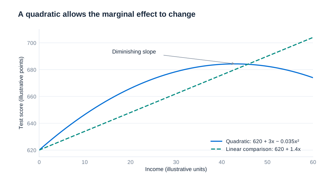
A quadratic should usually include both the linear and squared terms. Dropping the linear term imposes a zero slope at , an assumption that needs an economic justification. Centering income around a meaningful value can make the intercept and linear coefficient easier to interpret without changing fitted values, provided the corresponding transformed model includes all required terms.
Logarithms, proportional changes and skewness
The natural logarithm transforms multiplicative differences into additive differences. Its defining comparison is . Doubling a positive variable always increases its logarithm by , whether the original change is from 1 to 2 or from 100 to 200. This makes logs useful when proportional differences are more informative than absolute differences. Unless another base is explicitly stated, and here denote the natural logarithm, with base .
For a small proportional change , . Increasing income from 100 to 101 is a 1% increase and changes log income by approximately 0.01. Increasing it from 1 to 2 is a 100% increase and changes log income by approximately 0.693; treating this log difference as 1 would be a poor approximation. A log scale does not literally replace every difference by its percentage change. It expresses ratios in logarithmic units, which closely approximate proportional changes only when those changes are small.
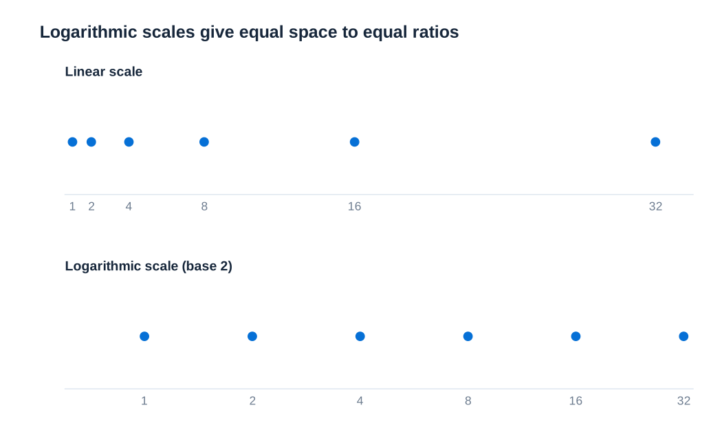
Logging a positive variable also compresses large values. Income often has a long right tail, and a histogram of log income may be more balanced than a histogram of income. However, logging does not guarantee normality, and normally distributed regressors are not an OLS requirement. The transformation should reflect the relationship being modelled and the interpretation required. It also changes the treatment of the data: the real-valued logarithm is undefined at zero and for negative observations. Adding an arbitrary constant before logging changes the model and must not be treated as an innocuous repair.
The linear–log model: outcome units for proportional input changes
When the outcome remains in levels but the regressor is logged, the model is:
The marginal effect in original units is , so an equal absolute increase in has a smaller fitted effect at higher starting values. A 1% increase in changes the fitted outcome by exactly , approximately units of . If is a test score and , a 1% income increase corresponds to approximately 0.2 score points, not a 20% increase in scores. The coefficient remains tied to the units of the outcome.
For any finite comparison from to , the fitted difference is . Doubling the regressor changes the fitted outcome by , not by . The latter would correspond to multiplying the regressor by . Changing the currency unit of a positive income regressor shifts its logarithm by a constant and changes the intercept, while leaving the slope and fitted differences unchanged.
This form is particularly useful when the raw relationship bends but the relationship between the outcome and log input appears closer to a straight line. It embodies a specific shape: with a positive coefficient, the outcome rises at a decreasing rate as the input increases. It cannot represent every possible pattern, such as a genuine U-shaped relationship, without additional terms.
Logged outcomes: semi-elasticities and elasticities
In a log–linear model, , a one-unit increase in changes the fitted log outcome by . The familiar interpretation, an approximately % change in , is accurate only for small coefficients. The exact proportional comparison implied by the fitted log values is:
for a change of units in . Thus a coefficient of 0.04 corresponds to about 4.08% for a one-unit increase, whereas a coefficient of 0.42 corresponds to about 52.20%, making the linear approximation much less satisfactory. A negative coefficient of −0.50 implies about 39.35% lower, not 50% lower.
Strictly, exponentiating a conditional mean of log outcomes describes a conditional geometric mean, not automatically the arithmetic conditional mean of the original outcome. From , the latter is . If the second factor differs across the observations being compared, exponentiating the fitted log difference alone does not give the arithmetic-mean ratio. This distinction matters when predicting expenditure totals or average earnings in currency units.
When both variables are logged, , the slope is an elasticity: . A small 1% increase in corresponds to an approximately % change in . For a finite proportional increase , the exact fitted proportional change is %. The log–log specification assumes a constant elasticity, whereas the log–linear specification assumes a constant semi-elasticity. These are substantive restrictions, not interchangeable ways of presenting the same regression.
Choosing a functional form
Model choice begins with the economic question, the units of measurement and the range of the observations. Scatterplots help identify curvature and influential observations; residual plots help reveal systematic patterns left unexplained by a fitted model. A skewed regressor may motivate considering a log transformation, but skewness alone does not establish that the conditional mean is linear in its logarithm. The same distinction applies to a skewed outcome: logging it changes the estimand and the weight given to proportional versus absolute errors.
Compare candidate models using the same observations when possible, check whether their implications are plausible within the data range, and consider predictive performance on observations not used for estimation. Ordinary values from a level-outcome regression and a log-outcome regression are not directly comparable measures of fit to the same dependent variable. A higher value after changing the outcome scale does not by itself establish a better model.
Interpretability is also valuable. A parsimonious specification that answers a clear question may be more useful than an elaborate curve with unstable behaviour. Report the marginal effects or fitted comparisons actually relevant to the application. In a quadratic model, give the income level at which a slope is evaluated; in a log model, distinguish a one-unit change from a 1% change. An attractive functional form still requires a credible identification strategy before its coefficients receive a causal interpretation.
Interactions and heterogeneous relationships
An additive model, , makes the slope with respect to one regressor independent of the other. That may be too restrictive. Rainfall may have a different association with traffic accidents when impaired driving is more common. Local economic conditions may alter the relationship between a governing party’s policy preferences and public spending. An interaction allows the slope to vary systematically:
The main coefficient is now the slope of when , while is the slope of when . The interaction coefficient measures how one slope changes as the other regressor increases. It should not be interpreted separately as the entire effect of either variable. Retaining both main effects generally avoids imposing arbitrary zero restrictions.
If is a binary indicator, compare predictions at and rather than imagining an infinitesimal change in group membership. In , the group difference is . Its uncertainty depends on both coefficient variances and their covariance:
Consequently, a confidence band for the combined effect cannot be reconstructed from the two reported standard errors alone. Interactions reveal heterogeneity in a fitted relationship; they do not themselves establish why that heterogeneity arises.
Worked example: education, experience and the gender wage gap
Consider a sample of 1,084 individuals from the US Current Population Survey. The outcome is the natural logarithm of hourly wage; education and experience are measured in years; equals 1 for women and 0 for men. Four nested regressions show how interpretation changes as controls and an interaction are added. The numbers in parentheses are standard errors. “Not included” means the regressor is absent from that specification, rather than that its coefficient was estimated as zero.
| Regressor | Model 1 | Model 2 | Model 3 | Model 4 |
|---|---|---|---|---|
| Education, years | 0.0692 (0.00556) | 0.0712 (0.00538) | 0.0874 (0.00562) | 0.0793 (0.00630) |
| Female indicator | Not included | −0.272 (0.0302) | −0.269 (0.0284) | −0.594 (0.147) |
| Experience, years | Not included | Not included | 0.0339 (0.00392) | 0.0347 (0.00391) |
| Experience squared | Not included | Not included | −0.000473 (0.0000847) | −0.000492 (0.0000843) |
| Female × education | Not included | Not included | Not included | 0.0253 (0.0116) |
| Observations | 1,084 | 1,084 | 1,084 | 1,084 |
Model 1 associates an additional year of education with approximately 6.92% higher hourly wages. Adding the female indicator in Model 2 changes that slope and introduces a conditional group comparison. Model 3 adds experience and its square. The positive experience coefficient and negative squared coefficient describe a concave experience profile: early additional experience has a larger fitted association than later additional experience. These changes illustrate why a coefficient is conditional on the rest of the specification; they do not identify which regression has solved all selection problems.
Model 4 allows the education slope to differ by gender. For men, the log-wage slope is 0.0793; for women it is . The exact fitted one-year proportional changes are approximately 8.25% and 11.03%, respectively, under the logged-outcome interpretation described above. The experience slope is . Its fitted turning point is about 35.26 years, whose substantive relevance depends on the observed support and the adequacy of the quadratic specification.
Interpreting and plotting the complete gender contrast
In Model 4, the female coefficient is not the wage gap for every education level. Holding experience constant, the fitted female-minus-male contrast in log wages at education level is:
At zero years of education, this implies a fitted geometric-mean wage ratio of , or about 44.79% lower, rather than 59.4% lower. Zero education may also lie far from most observations, making the intercept contrast a poor headline summary. At 12 years the fitted gap is approximately −25.20%; at 16 years it is −17.24%; and at 18 years it is −12.94%. These percentages use , not the large-coefficient approximation.
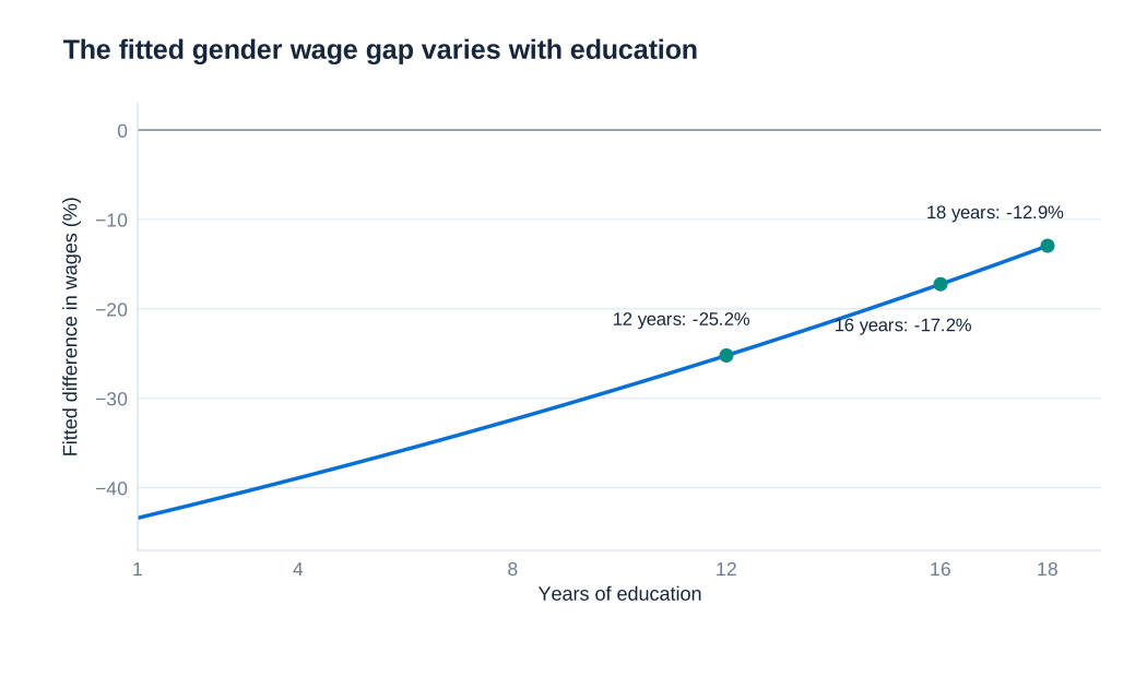
Each additional year of education raises the female-minus-male log-wage contrast by 0.0253. It does not close the exact percentage wage gap by a constant 2.53 percentage points, because exponentiation is nonlinear. Solving the fitted log contrast for zero gives about 23.48 years of education. That algebraic crossing extends beyond the 1–18-year range illustrated here and should not be interpreted as evidence that a particular amount of education eliminates wage inequality.
The regression documents conditional associations. Differences in occupation, hours, job tenure, employment selection and other unobserved characteristics can still affect the estimates. Nor does controlling for such variables automatically settle a discrimination question, since some controls may themselves reflect unequal opportunities. A useful empirical conclusion states precisely which wage measure, sample, controls and education level are being compared, and separates that comparison from any broader causal claim.
6. Dummy Variables and Binary Outcomes
Indicators, categories and the comparison they encode
A binary or dummy variable takes the value 1 when a defined condition holds and 0 otherwise. Employment status, an apartment’s ocean view and the presence of high blood pressure are examples. Binary variables are a special case of categorical variables, which classify observations into a limited set of groups. The coding must be stated explicitly: reversing 0 and 1 reverses the interpretation of the associated comparison.
A numeric category code is not necessarily a quantitative measurement. Coding blood types A, B, AB and O as 1, 2, 3 and 4 does not make type O “four times” type A, nor establish equally spaced biological differences. Treating these codes as one continuous regressor would impose an arbitrary ordering and constant steps. Separate indicators allow each group to have its own conditional mean relative to a chosen reference category.
There are two distinct uses of binary variables in regression. An indicator on the right-hand side represents a group comparison while leaving the nature of the outcome unchanged. An indicator on the left-hand side makes the conditional mean a probability, introducing restrictions that an ordinary straight line may fail to respect. The estimation principles remain connected, but the interpretation and appropriate diagnostics differ.
A dummy variable as an explanatory variable
Suppose monthly apartment rent, in currency units, is modelled using the number of rooms and an ocean-view indicator:
For a fixed room count, the fitted rent is without an ocean view and with a view. Thus is the conditional difference in monthly rent, measured in the same currency units as rent. The model assumes that this difference does not vary with the number of rooms. Adding would relax that restriction, allowing the view premium to vary with apartment size.
“Holding rooms constant” does not mean all other apartment characteristics are identical. If ocean-view properties also have better locations or higher construction quality and those variables are omitted, the coefficient may reflect those differences. The group indicator does not supply random assignment. Its coefficient is a conditional association unless the identifying assumptions justify more.
If the dependent variable is log rent, the coefficient changes meaning: the exact fitted proportional difference between view and no-view apartments is %, subject to the logged-outcome qualifications in Chapter 5. If an indicator interacts with another regressor, its standalone coefficient applies when that other regressor is zero, and the full group contrast must include the interaction.
Multiple categories and the dummy-variable trap
Consider a school-district example that groups computer availability into low, middle and high categories using the 25th and 75th percentiles. To define a complete classification, assign values below the 25th percentile to low, values from the 25th through the 75th percentile to middle, and values above the 75th percentile to high. Ties require a consistent boundary rule; the groups need not contain exactly 25%, 50% and 25% of observations.
Let and indicate middle and high availability. With low availability as the reference, estimate:
The intercept is the low group’s mean, and the two slopes are differences relative to it. Including all three group indicators together with an intercept produces perfect multicollinearity because their sum is exactly 1. This is the dummy-variable trap. Omitting one category with an intercept solves it; alternatively, omitting the intercept and retaining all categories estimates separate group means. Neither option discards observations from the reference group.
| Term | Coefficient | Standard error | t statistic | p value | 95% confidence interval |
|---|---|---|---|---|---|
| Middle versus low | 0.8566319 | 2.275697 | 0.38 | 0.707 | [−3.616636, 5.3299] |
| High versus low | −0.9260766 | 2.627719 | −0.35 | 0.725 | [−6.091303, 4.23915] |
| Intercept: low category | 653.9618 | 1.85367 | 352.79 | <0.001 | [650.3181, 657.6055] |
The fitted means are approximately 653.96 points for low availability, 654.82 for middle availability and 653.04 for high availability. Both difference intervals include zero. The joint test of the two category coefficients gives , with ; , adjusted , and the root mean squared error is 19.085 score points. These results provide little evidence of differences in this simple grouping. They do not prove that access to computers has no causal effect: the specification is an unadjusted group comparison, and the measure is computer availability rather than a randomly assigned intervention.
Binary outcomes and the linear probability model
For a binary outcome , its conditional expectation equals its probability of being 1: . Running OLS with a binary outcome therefore gives a linear probability model, or LPM. In , a one-unit increase in changes the fitted probability by , or percentage points. The scale is essential: a coefficient of 0.05 means five percentage points, not automatically a 5% relative increase.
For school districts, define when the district’s average test score is above the chosen overall average and 0 otherwise. A regression on average district income produces the following results. Income is kept in the dataset’s recorded units, so the slope applies to one unit on that scale; any currency conversion must be applied before interpreting a different unit change.
| Term | Coefficient | Robust standard error | t statistic | p value | 95% confidence interval |
|---|---|---|---|---|---|
| Average district income | 0.0328825 | 0.0029316 | 11.22 | <0.001 | [0.0271201, 0.038645] |
| Intercept | 0.0034945 | 0.0504409 | 0.07 | 0.945 | [−0.095655, 0.102644] |
There are 420 observations; , root mean squared error 0.44108, and the robust overall test is , with . A one-unit income increase is associated with about 3.288 percentage points higher probability of an above-average score. This comparison is about crossing a binary threshold, not the number of test-score points gained.
Probability bounds, heteroskedasticity and percentage points
A straight line need not stay between 0 and 1. The fitted school model is , which exceeds 1 when recorded income exceeds approximately 30.31. At , it predicts about 1.319, an impossible probability. Such predictions reveal a limitation of the functional form; merely truncating them to 1 does not change the model that was estimated or provide a principled marginal-effect calculation.
The LPM also imposes a constant probability slope. An income increase has the same fitted effect near a probability of 0.05 as near 0.95, although the room for further decreases or increases is very different. The importance of this restriction depends on the range of covariates and the purpose of the analysis. A linear approximation may be useful over a central range even if it behaves badly in the tails.
With a correctly specified conditional probability , the binary error variance is . It therefore generally varies with the regressors, making heteroskedasticity-robust standard errors appropriate. Robust inference addresses this variance problem; it does not repair impossible probabilities, omitted variables or an incorrect conditional mean. If observations are dependent within groups, the standard-error calculation must address that dependence as well.
Percentage points and percent changes answer different questions. A probability moving from 40% to 50% increases by 10 percentage points and by 25% relative to its starting value, because . In a group of fixed size 100, moving from 40 to 50 members with a characteristic illustrates both statements. Without a baseline probability, an LPM coefficient cannot be converted into a unique relative percentage change.
Probit, logit and maximum likelihood
Probit and logit replace the unrestricted probability line with a smooth cumulative distribution function. With an index , the probit model uses the standard normal cumulative distribution function :
The function is the area under the standard normal density to the left of . It maps every real-valued index into a probability strictly between 0 and 1 for finite values. The logit model uses the logistic function instead:
Both curves flatten near their lower and upper bounds. The raw coefficients describe changes in an index, not percentage-point changes in probability. For a continuous regressor without interactions, the probit marginal effect is , where is the standard normal density; the logit marginal effect is . Their magnitude depends on all covariates through the index. An average marginal effect averages these observation-specific derivatives, while an effect evaluated at average covariates is a different quantity.
For a binary regressor, calculate the discrete difference between predicted probabilities when its value is set to 1 and to 0, holding other covariates fixed. Interactions require still more care: the sign of a coefficient on a product term need not by itself equal the sign of every probability-scale interaction effect. Presenting fitted probabilities or explicitly calculated contrasts is often clearer.
These models are usually estimated by maximum likelihood rather than OLS. For independent observations with probabilities , the binary log-likelihood is:
Maximisation selects the parameter values that give the observed outcomes the greatest likelihood within the specified model. Probit, logit and LPM predictions can be similar over a central range, but this is not guaranteed, especially in the tails. Choose between them by considering the target comparison, predicted probability range, specification and interpretability. A nonlinear probability model supplies sensible bounds, not a causal research design.
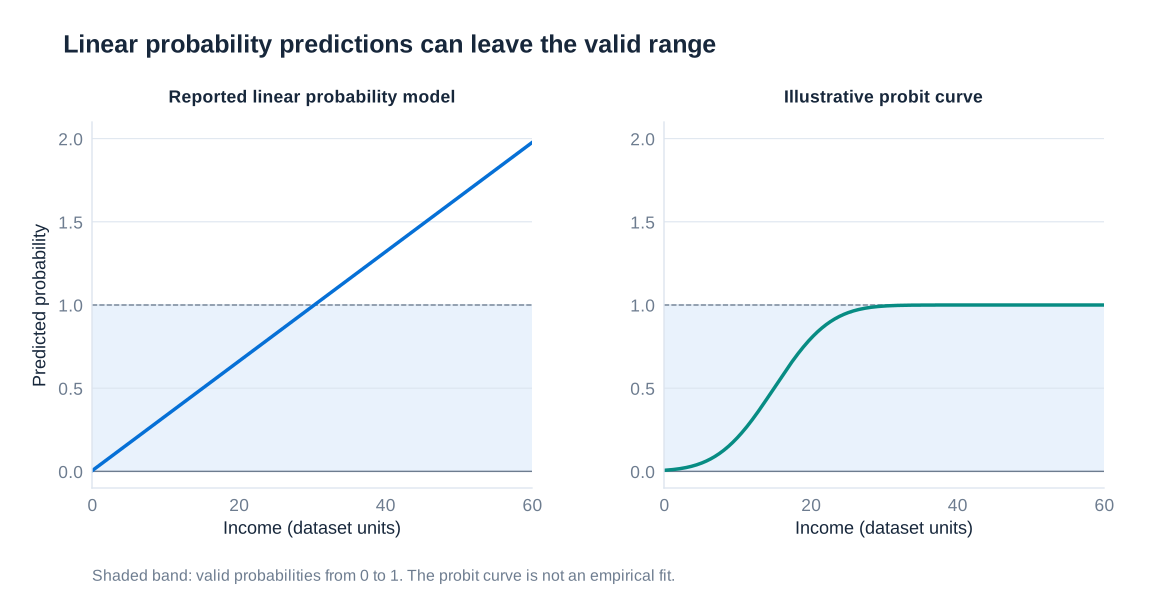
Reading a complete regression output
A coefficient table contains several distinct pieces of information. The coefficient gives an estimated conditional relationship in the model’s units. Its standard error measures sampling uncertainty under the chosen variance estimator. A test statistic compares the estimate with a hypothesised value, usually zero; the p value describes compatibility with that null under the testing assumptions. A 95% confidence interval summarises a range generated by a procedure with 95% long-run coverage. Neither the p value nor the interval measures the probability that a particular causal story is true.
The number of observations states the sample actually used. is the fraction of sample outcome variation explained by the fitted regression; adjusted penalises added regressors and may be negative. Root mean squared error expresses residual spread in the dependent variable’s units. The overall F test assesses a joint restriction on slope coefficients. None of these statistics substitutes for substantive effect sizes, a valid research design or a careful description of the sample.
| Conditional relationship | Comparison | Interpretation of the fitted change |
|---|---|---|
| One more unit of | units of | |
| One more unit of | Approximately %; exact fitted log-scale comparison % | |
| 1% more | Approximately outcome units; exactly | |
| 1% more | Approximately %; is the elasticity | |
| Binary , linear probability model | One more unit of | percentage points |
Logged-outcome comparisons refer directly to fitted log values and their implied geometric means; arithmetic-mean comparisons require the retransformation conditions discussed in Chapter 5. Every interpretation also holds the other included regressors fixed and remains associational unless additional assumptions establish causality.
Worked example: annual medical expenditure in levels
Three models use 2,970 observations and the same explanatory variables: age in years, the natural logarithm of personal income, and an obesity indicator equal to 1 for obese individuals and 0 otherwise. The first outcome is total annual medical expenditure measured in 2005 US dollars. Its coefficients therefore combine three interpretation rules: a level–level age effect, a level–log income effect and a discrete group difference.
| Term | Coefficient | Standard error | t statistic | p value | 95% confidence interval |
|---|---|---|---|---|---|
| Age, years | 202.1078 | 43.41592 | 4.66 | <0.001 | [116.9794, 287.2362] |
| ln(personal income) | −260.2222 | 772.2026 | −0.34 | 0.736 | [−1774.329, 1253.885] |
| Obese indicator | 1251.303 | 588.4134 | 2.13 | 0.034 | [97.56308, 2405.043] |
| Intercept | −4462.544 | 7241.433 | −0.62 | 0.538 | [−18661.29, 9736.197] |
Holding income and obesity status fixed, an additional year of age is associated with approximately USD 202.11 higher annual expenditure. A 1% income increase corresponds to approximately USD 2.60 lower expenditure, because the coefficient multiplies the change in log income; the exact fitted change is . The income estimate is very imprecise and its interval includes substantial positive and negative values, so the negative point estimate should not be presented as established evidence that income reduces expenditure.
At the same age and income, the obese group has fitted annual expenditure USD 1,251.30 higher. Its interval ranges from approximately USD 97.56 to USD 2,405.04. The intercept describes a non-obese individual at age zero and log income zero, meaning income equal to one in the recorded currency unit. This combination is generally not substantively representative; a negative intercept does not imply negative expenditure for a typical person.
The regression has , adjusted and root mean squared error 14,058 USD. The joint test gives , with . Statistical evidence of some association can coexist with low explanatory power and large individual prediction errors. The estimates do not isolate causal effects of ageing, income or obesity without further assumptions about omitted health conditions, selection and other determinants of expenditure.
Worked example: medical expenditure in logarithms
The second model uses the natural logarithm of annual expenditure. It therefore concerns proportional expenditure differences and requires positive expenditure observations for the logarithm to be defined. Although the reported sample size remains 2,970, one should never assume that an arbitrary dataset contains no zero expenditure merely because a logged specification is convenient.
| Term | Coefficient | Standard error | t statistic | p value | 95% confidence interval |
|---|---|---|---|---|---|
| Age, years | 0.0419183 | 0.0058171 | 7.21 | <0.001 | [0.0305124, 0.0533243] |
| ln(personal income) | −0.1696737 | 0.1034636 | −1.64 | 0.101 | [−0.3725414, 0.0331939] |
| Obese indicator | 0.420106 | 0.0788386 | 5.33 | <0.001 | [0.2655222, 0.5746899] |
| Intercept | 6.448543 | 0.9702434 | 6.65 | <0.001 | [4.546125, 8.350962] |
The age coefficient corresponds to approximately 4.19% higher expenditure per additional year, or an exact fitted geometric-mean difference of %. The income coefficient is an elasticity: a 1% income increase is associated with approximately 0.170% lower expenditure, holding age and obesity status fixed. The exact finite-change figure is about −0.169%. Its confidence interval includes zero and the p value is 0.101, so the data do not establish a nonzero income association at the conventional 5% level.
The obesity coefficient is large enough that the common small-coefficient approximation is misleading. The exact fitted difference is %, rather than 42%. This compares conditional geometric means. Describing it as a 52.21% difference in arithmetic mean expenditure would additionally require an appropriate retransformation assumption or calculation. The intercept is the fitted log expenditure for the baseline covariate combination, not expenditure in dollars.
The model reports , adjusted , root mean squared error 1.8836 log units and , with . Its cannot be compared directly with Model 1’s to decide which better predicts dollar expenditure, because the dependent variable and residual scale have changed.
Worked example: the probability of high blood pressure
The third outcome equals 1 if an individual has high blood pressure and 0 otherwise. OLS therefore estimates an LPM. The age and obesity coefficients describe probability differences; the income coefficient combines a probability outcome with a logged regressor.
| Term | Coefficient | Standard error | t statistic | p value | 95% confidence interval |
|---|---|---|---|---|---|
| Age, years | 0.0053784 | 0.001421 | 3.79 | <0.001 | [0.0025922, 0.0081646] |
| ln(personal income) | 0.0914678 | 0.0252735 | 3.62 | <0.001 | [0.0419125, 0.1410232] |
| Obese indicator | 0.1987462 | 0.0192582 | 10.32 | <0.001 | [0.1609854, 0.2365071] |
| Intercept | −0.6557299 | 0.2370055 | −2.77 | 0.006 | [−1.120442, −0.191018] |
An additional year of age is associated with percentage points higher probability. A 1% income increase changes the fitted probability by approximately , or 0.0914678 percentage points. Using the exact log change gives about 0.0910135 percentage points. Multiplying by 100 without also accounting for the 0.01 log change would overstate this comparison by a factor of 100.
The obese group has an estimated probability 19.87462 percentage points higher, conditional on age and income. This is not a 19.87% relative increase: the relative figure would require a specified baseline probability. The negative intercept illustrates again why a baseline outside the useful data range is not a plausible standalone probability. Predictions should be examined over the actual covariate values.
The output reports , adjusted , root mean squared error 0.46012 and , with . The displayed standard errors are conventional OLS standard errors, unlike the explicitly robust school-district example. Given the binary outcome, a sound empirical analysis should recompute heteroskedasticity-robust or otherwise appropriate uncertainty before relying on these reported tests. The coefficient interpretations remain as stated, but their statistical precision must be assessed using an adequate variance estimator.
7. Panel Data and Fixed Effects
A panel follows the same units over time. Its distinctive contribution is the ability to compare a person, firm, city or other unit with its own earlier observations. This changes the source of information used by a regression: persistent differences between units can be separated from changes within them. The distinction is valuable whenever an explanatory variable is correlated with stable characteristics that are difficult to measure. It does not, by itself, make an observational relationship causal.
What a panel records
Let identify units and identify periods. An observation is the outcome for unit in period ; is a time-varying explanatory variable. A city panel might record population, capital-city status and the presence of centres of higher learning at successive dates. Longitude is a time-invariant characteristic, written , because its value does not change within the same city. Capital-city status can change, so it belongs among the variables indexed by both and .
A balanced panel observes every unit in every period and contains observations. An unbalanced panel has different numbers of observations across units. This can reflect entry, exit, missing measurements or the historical availability of records. Unbalanced data are not automatically invalid: fixed-effects methods can use the available observations. However, selective disappearance matters. If a firm stops reporting precisely when an unobserved adverse shock occurs, analysing only its observed periods may introduce selection bias. The unit identifier must also remain consistent over time; a changed administrative boundary can create an apparent change that is partly a change in what is being measured.
Repeated cross-sections are different. Observing a new sample of workers every year permits comparisons of groups over time, but does not permit a within-worker transformation unless the same workers can be linked. A panel's repeated observations provide additional information, while also creating dependence: ten measurements of one person are not equivalent to ten independently sampled people.
Why pooled OLS can be misleading
Consider the additive model
The component collects all stable unit characteristics that affect the outcome, including unobserved ones. The idiosyncratic disturbance contains influences that vary over time. A pooled OLS regression that omits combines the two components into one error. Even if the time-varying disturbance is exogenous, a correlation between and creates omitted-variable bias. For instance, a city with a naturally favourable harbour may have both greater commercial activity and a larger population in every period. Comparing high-activity cities with low-activity cities mixes the association of activity with population and the persistent advantage of the harbour.
The key distinction is between between-unit variation, represented by differences in unit means, and within-unit variation, represented by deviations from each unit's own mean. A positive pooled relationship can coexist with a flat or negative within-unit relationship. Neither estimate should be interpreted without stating the comparison it uses. Fixed effects deliberately discard persistent level differences as a source of identification for .
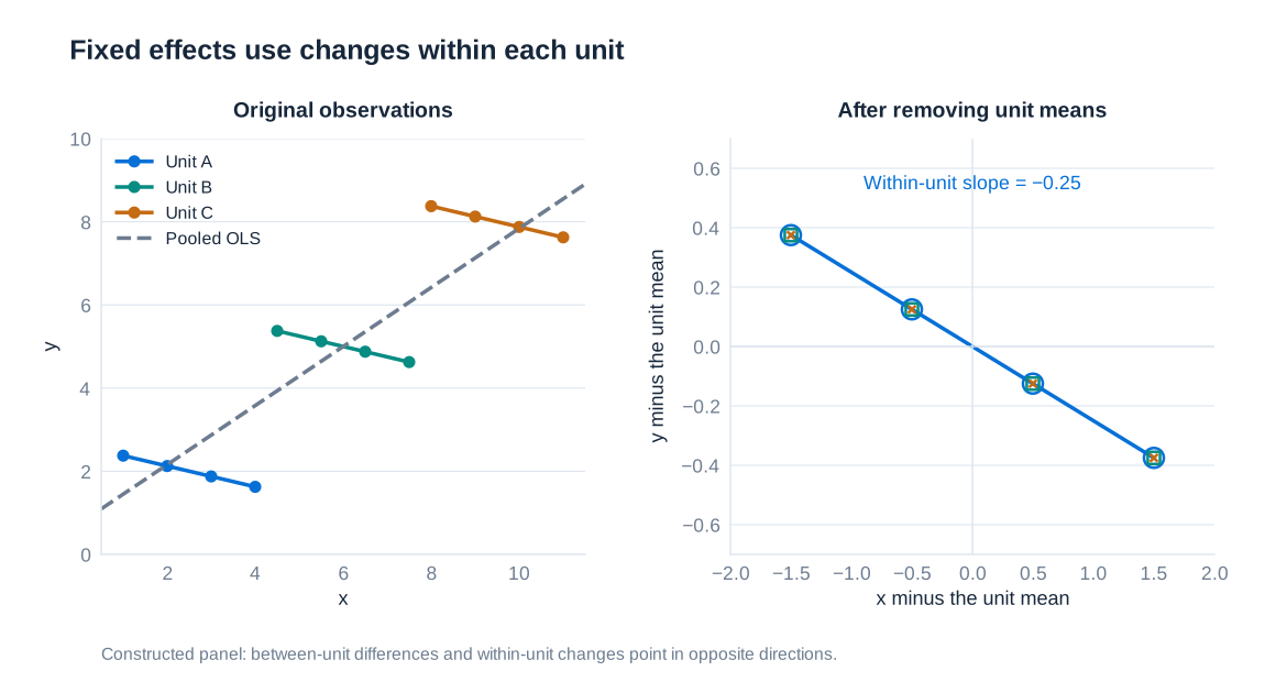
The within transformation
For a balanced panel, take each unit's time average. Define , and define and in the same way. The mean of is simply . Subtracting the averaged equation from the original equation gives
Both the common intercept and the unit-specific intercept disappear. OLS on these demeaned variables therefore estimates the slope without requiring to be uncorrelated with . For one explanatory variable, the within estimator is
The denominator shows a fundamental requirement: the explanatory variable must change within at least some units. A variable that is constant within every unit has a demeaned value of zero and cannot receive a separately identified coefficient. This is why a city fixed-effects regression cannot estimate a separate main effect of longitude. Its contribution is absorbed by the city intercept. A small amount of within-unit variation can also lead to imprecise estimates, even when the full dataset contains many observations.
For an unbalanced panel, the average for each unit is calculated over that unit's observed periods, using its own observation count . The algebra remains valid for a time-invariant additive effect. Appropriate assumptions about the observation process are still required for inference about the intended population.
Fixed effects as unit indicators
The same slope can be estimated by giving each unit its own intercept. With a common intercept, include unit indicators; the omitted unit supplies the reference intercept. Alternatively, include all indicators and omit the common intercept. Including both a common intercept and all unit indicators creates perfect multicollinearity because the indicators sum to one for every observation.
The least-squares dummy-variable regression and the within regression produce the same estimated slope when applied to the same observations and regressors. Software must also account correctly for the estimated fixed effects when constructing degrees-of-freedom adjustments. Choosing a different reference unit changes the interpretation of the intercept and indicator coefficients, but does not change fitted values or the slope of the time-varying regressor. Modern estimation routines absorb large collections of fixed effects rather than explicitly constructing thousands of indicator columns.
First differences
Another way to remove is to subtract the previous observation of the same unit:
The fixed effect cancels because . A first-difference regression asks whether a change in the explanatory variable accompanies a change in the outcome. One initial observation per unit is lost when constructing differences. If dates are missing, adjacent recorded rows must not automatically be treated as adjacent periods: a change over two years is not the same object as a one-year change.
With exactly two periods and the same sample, first differences and the within estimator yield the same slope. With more than two periods, both eliminate a fixed additive effect, but their estimates need not coincide. Their relative efficiency depends on the serial structure of the idiosyncratic disturbance. Differencing can also magnify the importance of measurement error when the true variable changes little over time. The choice should therefore reflect the economic model, data quality and error process.
Unit effects and period effects
A two-way fixed-effects model includes both unit and period intercepts:
Unit effects absorb stable differences across units: location, persistent infrastructure advantages or enduring characteristics of an individual. Period effects absorb shocks common to all units at a given date, such as a nationwide recession or a general technological change. For city populations, a common epidemic wave could be represented by a period effect only to the extent that its additive effect is shared across cities. A shock that hits ports more strongly than inland cities is not fully removed by one common time intercept.
In a balanced panel, subtracting unit means and time means and adding the overall mean removes both sets of intercepts. With unbalanced observations, this simple one-step double-demeaning formula is generally insufficient; an estimator that properly absorbs both effects is needed. Variables that move identically for every unit at each date are collinear with time effects. Identification consequently requires variation that remains after both sets of effects have been removed.
Exogeneity, serial dependence and inference
A standard sufficient condition for the static fixed-effects estimator is strict exogeneity of the idiosyncratic disturbance:
This condition permits correlation between the regressors and the stable effect , but rules out correlation between a disturbance in one period and regressors in any period. It is stronger than contemporaneous exogeneity. If an unexpected fall in city population causes the government to introduce a policy next period, the current shock is related to a future regressor. Removing the city mean does not remove this feedback. Time-varying omitted factors, simultaneous determination and endogenous measurement remain possible sources of bias. Lagged dependent variables require particular care in short panels because the within transformation generally makes them correlated with the transformed disturbance.
Repeated observations also create an inference problem. After fixed effects have been removed, idiosyncratic shocks can still be persistent within units. Cluster-robust standard errors allow heteroskedasticity and serial correlation within a specified cluster while relying on adequate independence across clusters. If policy varies by state, clustering only by individual can substantially understate uncertainty: many individuals share the same policy shock. The clustering level should follow the assignment mechanism and plausible common disturbances, and the number of independent clusters matters more than the raw number of rows. Clustered standard errors address uncertainty; they do not repair an endogenous regressor.
Random effects and the source of identifying variation
A random-effects model also separates from , but uses both within-unit and between-unit information. In its conventional form it requires the unit effect to be uncorrelated with the regressors at all dates, conditional on included controls. This assumption is demanding when, for example, unobserved management quality influences both a firm's investment and its output. If the assumption is credible, random effects can improve efficiency and estimate coefficients on time-invariant regressors that fixed effects absorb.
Random effects are therefore a substantive modelling choice, not an obsolete method. Correlated random-effects approaches can relax the conventional assumption by explicitly including functions of a unit's regressor history, such as time averages. A comparison of fixed- and random-effects estimates can be informative, but an automated test cannot establish the economic credibility of all identifying assumptions. Above all, a table containing coefficients for time-invariant geography cannot be described as a standard city fixed-effects regression that also estimates those geography main effects.
Long-run city development: reading an empirical table
Bosker, Buringh and van Zanden's study of urban development between 800 and 1800 assembles information on 793 cities across Europe, the Middle East and North Africa. The setting distinguishes stable geography from changing institutions. Sea access and transport networks can influence commerce, while political and religious status can change a city's administrative or economic role. Historical coverage and variable availability mean that individual regression samples need not contain every city at every date.
The following baseline table is a random-effects specification with additional ecozone, country and century fixed effects. It is not the city fixed-effects specification developed above. The dependent variable is the natural logarithm of city population. Each reported cell gives a coefficient followed by its city-clustered p-value in brackets. A displayed p-value of 0.00 is a rounded small value, not a probability known to be exactly zero. “Not included” identifies a variable not estimated in that specification rather than a missing result.
| Characteristic | All cities | Muslim cities | Christian cities | Middle East / North Africa | Europe | Muslim cities: Middle East / North Africa | Christian cities: Europe |
|---|---|---|---|---|---|---|---|
| Sea access | 0.25*** [0.00] | 0.24 [0.11] | 0.25*** [0.00] | 0.42*** [0.01] | 0.26*** [0.00] | 0.38** [0.04] | 0.25*** [0.00] |
| River access | 0.09** [0.04] | 0.12 [0.23] | 0.05 [0.31] | 0.21* [0.07] | 0.06 [0.25] | 0.11 [0.42] | 0.05 [0.3] |
| Roman road | 0.03 [0.59] | −0.09 [0.55] | 0.06 [0.22] | 0.08 [0.71] | 0.03 [0.61] | 0.05 [0.84] | 0.05 [0.28] |
| Roman-road hub | 0.09* [0.10] | 0.08 [0.54] | 0.10** [0.04] | 0.12 [0.55] | 0.08 [0.13] | 0.12 [0.57] | 0.10** [0.05] |
| Caravan route | 0.08 [0.46] | 0.31* [0.05] | −0.34*** [0.00] | 0.06 [0.66] | Not included | 0.25 [0.15] | Not included |
| Caravan hub | 0.5*** [0.00] | 0.78*** [0.00] | 0.09 [0.61] | 0.55*** [0.00] | Not included | 0.70*** [0.00] | Not included |
| Bishopric | 0.18*** [0.00] | 0.22** [0.04] | 0.19*** [0.00] | 0.37*** [0.00] | 0.17*** [0.00] | 0.27* [0.06] | 0.19*** [0.00] |
| Archbishopric | 0.34*** [0.00] | 0.12 [0.45] | 0.41*** [0.00] | 0.35 [0.16] | 0.39*** [0.00] | 0.22 [0.36] | 0.41*** [0.00] |
| Christian holy city | 0.26 [0.26] | Not included | 0.47 [0.12] | 0.29 [0.57] | 0.22 [0.54] | Not included | 0.34 [0.34] |
| Muslim holy city | 0.19 [0.24] | −0.08 [0.79] | Not included | 0.02 [0.93] | Not included | −0.18 [0.62] | Not included |
| Capital city | 0.87*** [0.00] | 0.67*** [0.00] | 0.93*** [0.00] | 0.73*** [0.00] | 0.91*** [0.00] | 0.72*** [0.00] | 0.95*** [0.00] |
| Centre of higher learning | 0.32*** [0.00] | 0.09 [0.83] | 0.30*** [0.00] | 0.11 [0.75] | 0.29*** [0.00] | 0.16 [0.74] | 0.30*** [0.00] |
| Madrasa | 0.25** [0.01] | 0.12 [0.25] | Not included | 0.19 [0.11] | 0.12 [0.48] | 0.16 [0.19] | Not included |
| Plundered | 0.03 [0.56] | 0.02 [0.57] | −0.09 [0.14] | 0.07 [0.103] | −0.16*** [0.01] | 0.03 [0.41] | −0.14** [0.03] |
| Log Muslim urban potential | 0.08 [0.31] | 0.30** [0.04] | 0.03 [0.72] | 0.24 [0.12] | 0.19** [0.04] | 0.29* [0.10] | 0.07 [0.47] |
| Log Christian urban potential | 0.23*** [0.00] | 0.29 [0.12] | 0.25*** [0.00] | −0.02 [0.9] | 0.21*** [0.00] | 0.18 [0.43] | 0.25*** [0.00] |
| R² | 0.46 | 0.52 | 0.43 | 0.60 | 0.40 | 0.56 | 0.41 |
| Observations | 2,596 | 656 | 1,940 | 570 | 2,026 | 499 | 1,869 |
Dependent variable: natural log of city population. Brackets contain p-values based on standard errors clustered by city. Significance markers are reproduced at their reported precision: * 10%, ** 5%, *** 1%. All specifications allow city random effects and include ecozone, country and century fixed effects. Additional controls cover religion where applicable, relevant logged distances to Mecca, Byzantium and Rome, log elevation, log surrounding ruggedness and cultivation potential. The centre-of-higher-learning indicator and madrasa indicator distinguish the two institutional categories used in the study.
Transport patterns differ across subsamples: sea access has a positive association in most specifications, while caravan networks have especially strong associations in Muslim-city samples. The measures of urban potential distinguish access to Muslim and Christian city networks; their log coefficients are elasticities conditional on the model. Capital status is positively associated with population throughout the table. Religious administrative status and centres of learning also show positive associations in several samples. These findings describe conditional relationships, not automatic proof of causal institutional effects. A growing city may acquire a political or educational institution because it is already expanding.
The interpretation depends on functional form. A capital coefficient of 0.87 corresponds to a fitted population ratio of , or about 139% more in the exponentiated log specification, rather than 87% exactly. For a log urban-potential variable, a coefficient of 0.23 instead means that a 1% change in urban potential is associated approximately with a 0.23% change in population. Such exponentiation describes fitted ratios on the log scale; translating them into arithmetic conditional mean populations can additionally require a retransformation adjustment when the disturbance distribution changes across observations.
Interpreting time indicators correctly
With the year 800 omitted, a century coefficient compares a period with that reference period, conditional on the other regressors. The table below is a coefficient-interpretation example. Its stated sample has 8,723 observations, so it must not be conflated with the 2,596-observation baseline above. Only reported centuries are listed; no estimates are supplied for omitted entries in the example.
| Century | Log coefficient | t-statistic |
|---|---|---|
| 800 | Reference period | Not estimated |
| 900 | 0.299 | 1.89 |
| 1000 | 0.845*** | 5.35 |
| 1100 | 0.963*** | 6.10 |
| 1200 | 1.553*** | 9.83 |
| 1300 | 3.006*** | 19.03 |
| 1400 | 2.224*** | 14.08 |
| 1700 | 4.955*** | 31.37 |
| 1800 | 8.036*** | 50.87 |
Year 800 is the omitted category. The example does not report coefficients for 1500 or 1600. Three stars denote significance at the 1% level.
In a log-outcome model, is a small-coefficient approximation to a percentage difference. The exact exponentiated comparison is . Thus 0.299 implies approximately 34.9%, while 0.845 implies approximately 132.8%. At 8.036, the approximation is entirely inappropriate: the corresponding fitted ratio is about 3,090.2, not a population difference of 803.6%. The exceptionally large value illustrates why a result's scale and provenance must be checked before giving it a substantive historical interpretation.
Changing effects of geography and institutions
Although the main effect of a time-invariant characteristic is absorbed by unit effects, its interaction with time can be identified. Suppose records coastal access. In a city and time fixed-effects model, include interacted with each period indicator except the reference year. A coefficient then measures how the coastal–inland difference changed relative to that reference year, rather than the overall difference in that year.
| Century | Interaction coefficient |
|---|---|
| 800 | Reference period |
| 900 | 0.14 |
| 1000 | 0.09 |
| 1100 | 0.02 |
| 1200 | −0.03 |
| 1300 | 0.12 |
| 1400 | 0.02 |
| 1500 | 0.11 |
| 1600 | 0.27 |
| 1700 | 0.38** |
| 1800 | 0.45** |
City and period fixed effects are included. Two stars denote significance at the 5% level. Standard errors and t-statistics are not provided in this example.
The coefficient 0.45 for 1800 is an additional 0.45 log points in the coastal–inland gap relative to 800. Exponentiating gives a ratio-of-ratios of , or about a 56.8% increase in that relative ratio. It is not automatically a 45-percentage-point difference in ordinary population growth rates. Such a percentage-point statement would require additional information about the baseline and growth rates being compared.
A time-varying characteristic can be interacted with all period indicators when the separate overall main effect is omitted and the design matrix has sufficient rank. For capital status, this parameterization estimates a period-specific coefficient directly. If instead one includes an overall capital coefficient plus interactions for all but the reference period, the interactions become deviations from that reference coefficient. These are alternative parameterizations of the same fitted relationships, not competing economic theories.
| Century | Capital-status coefficient |
|---|---|
| 800 | 0.19 |
| 900 | 0.50 |
| 1000 | 0.41 |
| 1100 | 0.40*** |
| 1200 | 0.48*** |
| 1300 | 0.47*** |
| 1400 | 0.45*** |
| 1500 | 0.61*** |
| 1600 | 0.63** |
| 1700 | 0.82** |
| 1800 | 0.64* |
City and period fixed effects are included. Significance: * 10%, ** 5%, *** 1%. Standard errors and t-statistics are not provided in this example.
For example, a period-specific capital coefficient of 0.64 corresponds to an exponentiated conditional difference of about 89.6%. Whether this deserves a causal interpretation still depends on why capital status changed and whether relevant time-varying confounders were controlled. Interactions expand the model's flexibility, but they do not create exogenous variation.
Evaluating a panel result
A useful assessment begins by identifying the unit, period and actual estimation sample. It then asks which variables change within units, which effects are absorbed, and what remaining variation identifies the coefficient. The economic story must explain why that variation is unrelated to the idiosyncratic disturbance. Finally, the uncertainty calculation must respect the dependence induced by repeated observations and shared shocks. Panel data help remove a specific class of omitted variables—stable additive unit characteristics—but a credible causal design must also address the confounders that remain.
8. Difference-in-Differences
Difference-in-differences, usually abbreviated DiD, estimates an effect by comparing an outcome's change in a treated group with its change in a comparison group. It uses two dimensions of variation: differences across groups and differences across time. Its central question is whether the comparison group's evolution can reveal what would have happened to the treated group without treatment. The method is especially useful when a policy changes in one place or for one group while a credible comparison remains untreated.
Why a double difference is needed
A before-and-after comparison within a treated group combines the effect of treatment with everything else that changed over time. An increase in agricultural yields following a reform may partly reflect better weather or new seed varieties. A treated-versus-control comparison after the reform has a different problem: the groups may have differed before any reform occurred. DiD subtracts the comparison group's change from the treated group's change, removing a common time change as well as a stable pre-existing group difference.
Write for the treated group, for the comparison group and and for periods before and after treatment. The sample estimator is
Equivalently, it is the post-treatment difference between the groups minus their pre-treatment difference. This arithmetic is always possible when the four means exist. Whether its result is a causal effect depends on assumptions about the unobserved counterfactual. A regression command cannot supply those assumptions.
A complete calculation: tenancy reform and rice yields
Operation Barga, introduced in West Bengal in 1978, sought to regulate tenancy rents and strengthen sharecroppers' security. Improved security and a greater retained share of output could change effort, investment and bargaining incentives. A familiar illustration associated with Banerjee, Gertler and Ghatak's work compares rice yields in West Bengal with those in neighbouring Bangladesh, which did not receive the same reform. The outcome is measured in kilograms per hectare, so differences retain that unit.
| Group | Before reform | After reform | Change |
|---|---|---|---|
| West Bengal | 1,308 | 1,650 | 342 |
| Bangladesh | 1,297 | 1,562 | 265 |
| West Bengal minus Bangladesh | 11 | 88 | 77 |
The treated group's increase is kg/ha. The comparison group's increase is kg/ha. Their difference is therefore kg/ha. The same answer follows from . Using only the treated group's increase would attribute all 342 kg/ha to the reform. Using only the final group difference would produce 88 kg/ha and ignore the initial gap.
The counterfactual post-reform yield for West Bengal is its initial yield plus the comparison group's increase:
The estimated effect is the vertical gap between actual yield, 1,650, and counterfactual yield, 1,573: precisely 77 kg/ha. The control group's actual final yield is 1,562, which is not the treated group's counterfactual because their initial levels differed. Relative to the estimated counterfactual, 77 kg/ha is about 4.9%; relative to initial treated yield, it is about 5.9%. These percentages answer different questions and must be labelled accordingly. Four means suffice to compute a point estimate, but do not supply a standard error or establish that the identifying assumptions hold.
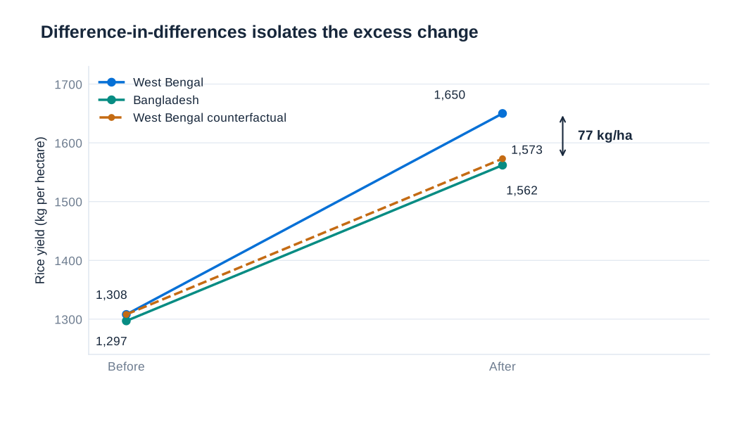
Parallel trends is a counterfactual assumption
Let denote the outcome that unit would have without treatment, and the outcome under treatment. Let indicate membership in the treated group. Parallel trends requires equal average changes in untreated potential outcomes:
This does not require equal initial outcome levels. It also does not require observed outcomes to remain parallel after treatment; a treatment effect is exactly what may make observed paths diverge. The assumption concerns the path the treated group would have followed without treatment. That path is unobserved after treatment begins, which is why parallel trends cannot be directly verified from the post-treatment data.
Under no anticipation and an untreated comparison group, the observed DiD equals the average treatment effect on the treated plus the difference in their untreated trends. Parallel trends sets the latter term to zero. This identifies an effect for the treated population, not necessarily the effect that would arise if every other group adopted the same policy. Similar geography or similar baseline means can help justify a comparison, but neither property guarantees similar counterfactual changes.
Anticipation, spillovers and composition
No anticipation means that behaviour before the designated treatment date has not already responded to the impending policy. If a reform is announced in advance and farmers begin investing immediately, treating the announcement-to-implementation period as an unaffected baseline can distort the estimate. The relevant treatment date should reflect when behaviour could change.
No interference across comparison groups requires careful thought about spillovers. A neighbouring region may be attractive as a control because it faces similar conditions, yet trade, migration or policy competition can transmit the treatment into that region. If the comparison group's outcome also responds, the estimated contrast is generally not the treated group's effect relative to a fully untreated world.
Group composition must also remain suitable for the comparison. In repeated cross-sections, different people may be observed before and after, and treatment-induced migration or survey nonresponse can change the population represented by a group mean. A panel reduces some composition concerns but can still suffer selective attrition. Time-varying covariates may improve a conditional comparison when they are appropriate confounders; controlling for a variable caused by the treatment can instead remove part of the effect being estimated or introduce bias.
The two-group, two-period regression
The elementary DiD can be estimated by an interaction regression:
Here after treatment and zero before. The intercept is the comparison group's pre-treatment mean. The coefficient is the treated group's initial difference from that mean. The coefficient is the comparison group's change over time. The interaction captures the treated group's additional change. These statements follow by setting the two indicators to zero or one in each of the four cells.
| Quantity | Regression expression | Value (kg/ha) |
|---|---|---|
| Comparison group, before | 1,297 | |
| Treated group, before | 1,308 | |
| Comparison group, after | 1,562 | |
| Treated group, after | 1,650 | |
| Initial group difference | 11 | |
| Comparison-group change | 265 | |
| Additional treated-group change | 77 |
The saturated regression reproduces the four sample cell means and the same DiD point estimate. If weights or additional regressors are introduced, the resulting estimate reflects those choices and need not equal the simple unweighted four-mean contrast. A coefficient in kilograms per hectare remains an absolute yield effect; a log-outcome model would instead require interpretation on the log scale and an explicitly justified transformation.
Many units, many periods and treatment intensity
With many units and periods, fixed effects provide a convenient regression representation:
Unit effects replace a single average treated-versus-control level difference with an intercept for each unit. Period effects replace a single post indicator with an intercept for each date. The treatment variable records actual exposure in that unit and period. This flexibility is useful, but it does not mean every two-way fixed-effects coefficient automatically estimates a well-defined average causal effect.
Minimum legal drinking-age policies illustrate why treatment need not be binary or start at a common date. Following the end of US Prohibition, states set different age rules; several lowered their thresholds during the early 1970s. In the historical comparison, Alabama lowered its threshold to 19 in 1975, Arkansas retained 21, and Tennessee lowered it to 18 in 1971 before raising it to 19 in 1979. Later federal policy encouraged a minimum age of 21, adopted in every state by 1988. These changes create variation in the fraction of young adults legally able to purchase alcohol.
Define as the proportion of 18–20-year-olds in state and year who are legally eligible. A model for their mortality rate can be written as
When is coded between zero and one and is deaths per 100,000 people, describes the fitted difference associated with moving from none to all of the age group being eligible. A 10-percentage-point increase in eligibility corresponds to . The model imposes a linear relationship in treatment intensity; stronger assumptions are needed to interpret differences across doses causally. State effects absorb fixed state differences and year effects absorb common annual shocks, while simultaneous policy changes or differential mortality trends can still confound the estimate.
Pre-treatment evidence and event studies
Several pre-treatment periods make a research design more informative because they reveal whether the groups were already moving differently. For a common treatment date , an event-study specification replaces one post-treatment coefficient with treatment-group interactions for relative dates:
The period immediately before treatment, , is omitted as the reference. Pre-treatment coefficients measure how the treated–comparison gap at earlier dates differs from that reference gap. Post-treatment coefficients describe how the gap evolves after exposure. Plotting point estimates with appropriate uncertainty intervals makes timing, precision and persistence easier to assess than a single average coefficient.
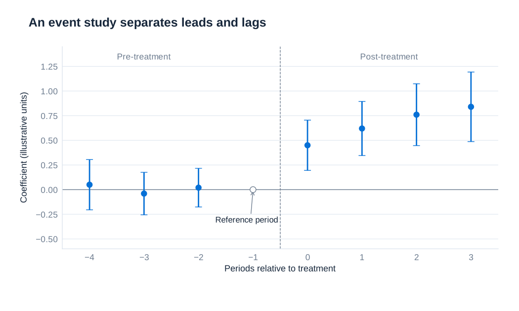
Pre-treatment estimates near zero are consistent with parallel trends, but do not prove the assumption. A test can have low power, confidence intervals can permit economically substantial differences, and a new post-treatment shock may affect the groups differently despite similar histories. Conversely, significant pre-treatment differences may reveal anticipation, an unsuitable comparison group or misspecification. Both individual estimates and a joint test of pre-treatment coefficients are informative, alongside substantive knowledge of the setting. The credibility claim concerns counterfactual post-treatment trends, so a nonsignificant pretrend test must never be presented as conclusive validation.
Differential trends and their limits
A conventional DiD fails when treated and comparison units would have continued along different trends without treatment. One sensitivity specification adds unit-specific linear trends:
The coefficient permits each unit to have a stable linear deviation from the common time path. The treatment coefficient then reflects departures from those fitted paths. This replaces simple parallel trends with a stronger functional-form claim about how untreated differences would have evolved. It is not a general repair for any arbitrary divergence.
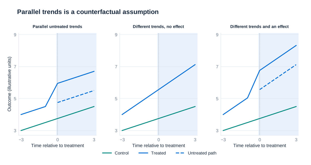
Three cases clarify the distinction. With parallel untreated paths and a discrete treatment-induced jump, a standard DiD can recover the jump. With nonparallel untreated paths and no treatment effect, the changing group gap can produce a spurious DiD. With nonparallel paths plus a genuine jump, a correctly specified differential-trend model may separate the discontinuity from smooth pre-existing divergence. However, if treatment effects emerge gradually, fitting unit-specific trends to all periods can absorb part of the effect. Conclusions should therefore consider how trend estimates, treatment dynamics and the chosen pre-treatment window interact.
Staggered adoption and heterogeneous effects
When units adopt treatment at different dates and effects vary across cohorts or exposure durations, a conventional two-way fixed-effects regression can use already-treated units as controls for newly treated units. The resulting coefficient can combine comparisons with difficult or even negative weights and need not equal the intended average treatment effect on the treated. A clean elementary DiD interpretation should not be carried over automatically.
Modern approaches estimate effects for treatment cohorts and dates using suitable never-treated or not-yet-treated comparison units, then aggregate those effects transparently. The researcher must define the target population and weighting scheme, justify parallel trends and no anticipation for the selected comparisons, and identify which post-treatment horizons have credible controls. Reversible policies and continuous treatment require additional care because methods designed for a single absorbing adoption date do not automatically apply.
Uncertainty and the effective amount of information
Outcomes and policy exposures often persist over time. Treating every person-year or state-year as independent can make standard errors much too small. In a state-policy design, clustering by state allows disturbances to be correlated across years and across observations sharing that state. If important shocks cross state boundaries, state clustering alone may not capture the entire dependence structure. The appropriate level follows the research design and the plausible correlation of the disturbances.
More observations inside the same few policy units do not create many independent policy experiments. The relevant issue is the number and balance of independent clusters, especially the number receiving treatment. There is no universal threshold at which cluster-robust inference becomes automatically reliable. With few clusters, methods such as suitable small-sample corrections, wild-cluster bootstrap procedures or design-based randomization inference may be needed, with assumptions explained. The four aggregate rice-yield means, for example, cannot alone justify a conventional standard error. A complete DiD study combines transparent arithmetic, a defensible counterfactual and an uncertainty calculation matched to the actual assignment structure.
9. Legal Status and Political Representation
Public policy can alter political participation without immediately changing who is legally entitled to vote. Immigration legalization provides a particularly revealing example: removing uncertainty about residence and employment may change household investment, civic engagement and the capacity of an existing community to support political candidates. This chapter examines Bernini and Sabet’s study of the Immigration Reform and Control Act (IRCA). It connects treatment intensity, fixed effects, event studies, instrumental variables and mechanism analysis within one empirical investigation. The outcome called political mobility is advancement between elected offices; it does not mean geographical migration or movement between jobs.
Legalization before widespread enfranchisement
IRCA was enacted in 1986 and enabled nearly three million undocumented immigrants to obtain legal status. Approximately 86 percent of applicants were Hispanic. Permanent residence began to be granted in 1989, while the usual five-year wait before naturalization separated legalization from the acquisition of citizenship and voting rights. The main political analysis therefore concentrates on 1984–1994. This timing creates a useful distinction between the consequences of more secure legal status and those of directly adding newly naturalized voters to the electorate.
People lacking legal status were already residents and were included in population statistics. Legalization therefore changed the legal composition of the existing population rather than mechanically adding the same number of new residents. This is an institutional argument, not a guarantee that migration or other demographic responses were absent. Those responses must be examined empirically. Nor does the timing imply that every political change before 1995 was entirely free of naturalization: the defensible claim concerns the period before widespread naturalization of IRCA beneficiaries.
The political mechanism is broader than recipients casting ballots. Security against removal and permanent access to employment may encourage educational investment, make families more willing to contact public institutions, and strengthen organizations serving mixed-status households. Relatives and other community members who already hold voting rights can respond. An increase in Hispanic officeholders is consequently compatible with most newly legalized residents remaining ineligible to vote during the main observation window.
Measuring exposure and matching the unit of analysis to the question
The treatment is a continuous county-level measure. The researchers count IRCA applicants relative to the county population in 1980, multiply by 1,000, and standardize the resulting variable. A one-unit change in the standardized measure means one standard deviation of exposure across counties. It does not mean one additional applicant, one percentage point of the population, or that every resident receives treatment.
Writing the unstandardized exposure as and its standardized form as makes the units explicit:
Administrative records contain 3,039,239 applicants, of whom 2,744,173 have county identifiers. The remaining 295,066 retain state identifiers, but their county information is suppressed. Allocating these observations across counties introduces a measurement issue rather than merely a data-cleaning inconvenience: different allocation rules can change the intensity measure. The study therefore repeats the analysis with alternative imputation procedures, denominators and predictions.
Political representation comes from a newly assembled longitudinal database of Hispanic elected officials. For aggregate representation, the unit is an office category within a county and year. For career progression, it is an individual official and year. School enrollment, teacher employment, political participation and fiscal outcomes draw on additional administrative and survey sources. These datasets answer different questions and need not contain the same observations. A larger number of individual records does not create an equally large number of independent treatment assignments because exposure varies at county level.
A continuous-treatment difference-in-differences design
The baseline specification compares changes in outcomes between places with different IRCA exposure, before and after permanent residence began to be granted:
Here denotes the observation unit, its county and its state. The unit fixed effect absorbs stable differences between counties, schools or politicians, depending on the outcome. State-by-year effects absorb shocks shared within a state in a particular year. Baseline county characteristics , interacted with the post-treatment indicator, allow the post-period change to differ with pre-existing demographic and economic conditions. Standard errors are clustered by county because both the exposure and plausible unobserved shocks are shared within counties.
The identifying condition is a conditional parallel-trends assumption: absent legalization, outcome changes would not have varied systematically with baseline IRCA intensity after accounting for the included controls and fixed effects. The comparison is between more- and less-exposed places, not between randomized recipients and nonrecipients. The coefficient describes the differential outcome change associated with one standard deviation of county exposure under this model. Interpreting it as the individual effect of granting one person legal status would change both the estimand and the unit of treatment.
An event study replaces the single post interaction with year-specific exposure interactions and omits 1988 as the reference year. Its coefficients measure differences relative to that baseline. For outcomes available only at long intervals, a long-difference regression relates the change in the outcome to exposure, baseline controls and state fixed effects. These alternatives retain the central comparison while adapting it to the observation frequency.
What the representation estimates actually measure
The representation outcome divides the number of Hispanic officeholders by the total number of seats in the same office category and county measured in 1987. Keeping this denominator fixed helps separate changes in Hispanic representation from changes in the number of available offices. The following results use the July 2026 research paper consistently. Effects and standard errors are in percentage points for a one-standard-deviation increase in county exposure; the baseline means are percentages.
| Office category | Effect, percentage points | County-clustered standard error | Pre-1989 mean, percent |
|---|---|---|---|
| All local elected offices | 0.488 | 0.141 | 1.226 |
| All local governing boards | 0.613 | 0.211 | 1.418 |
| School boards | 0.997 | 0.334 | 1.488 |
| All city offices | 0.737 | 0.263 | 1.350 |
| City governing boards | 0.603 | 0.253 | 1.335 |
| All county offices | 0.000 | 0.141 | 0.876 |
| County governing boards | −0.148 | 0.333 | 1.479 |
The school-board coefficient is approximately one percentage point. Relative to the baseline mean, . The corresponding city-board calculation is . Neither number means that representation rose by 67 or 45 percentage points. The county-level estimates are too imprecise to establish comparable gains. The pattern suggests expansion at school and city institutions, where entry points into elected office are more numerous.
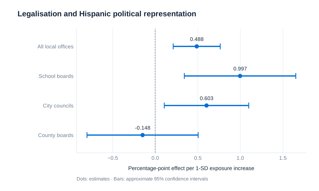
The event-study estimates strengthen the timing argument. The pre-1989 coefficients are jointly indistinguishable from zero, while representation increases gradually after legalization: approximately 0.4 percentage points by 1990, 0.8 by 1992, and 1.3–1.4 by 1994 for the combined school-and-city-board outcome. These dynamic estimates concern a combined outcome and should not be substituted for the separate school-board coefficient in the table. Gradual increases across election cycles are consistent with political incorporation rather than an immediate relabeling of existing officials. A pre-trend test cannot prove that the unobserved counterfactual would have remained parallel.
Following the same politician over time
Aggregate gains could reflect more entrants into office, advancement of existing politicians, or both. To study careers, the researchers follow Hispanic officials and code whether they move between government levels from one year to the next. The dependent variable equals 100 for a transition and zero otherwise, so regression coefficients directly express percentage-point changes in transition probabilities. Individual fixed effects remove stable differences in ambition or ability, but they do not absorb time-varying opportunities or shocks.
| Outcome | Effect, percentage points | Clustered standard error | Baseline probability, percent |
|---|---|---|---|
| Any upward move, all offices | 0.280 | 0.117 | 0.804 |
| Any downward move, all offices | −0.011 | 0.053 | 0.687 |
| Upward move among governing boards | 0.426 | 0.096 | 0.557 |
| School board to city board | 0.317 | 0.135 | 0.582 |
| City board to county board | 0.066 | 0.035 | 0.129 |
For upward moves among governing boards, the relative increase computed from the reported entries is . The absolute increase remains 0.426 percentage points: a large relative change can arise from a small initial probability. For all offices, the analogous calculation is about 34.8 percent. Using the displayed table entries avoids misleading percentages obtained by dividing heavily rounded numbers.
The clearest advancement occurs from school boards to city boards. The smaller city-to-county estimate has weaker precision, and the data do not establish a general expansion of jumps to state or federal office. There is also no clear increase in downward mobility. Together, these results support an interpretation of upward progression through nearby institutional levels, rather than indiscriminate turnover across the political hierarchy.
Historical settlement as an instrument
County exposure may remain correlated with unobserved local conditions. The instrumental-variable strategy uses the 1970 share of agricultural workers who were Hispanic, interacted with the post-1989 indicator, to predict exposure. Historical agricultural settlement and migrant networks help explain why some counties later had more eligible applicants. IRCA’s agricultural-worker provision makes this connection particularly relevant.
The first stage predicts the endogenous exposure interaction from the historical settlement interaction and the same exogenous covariates and fixed effects. The second stage replaces the exposure interaction with its fitted component. Two-stage least squares uses only variation in exposure associated with the instrument. In the baseline representation specification, the reported second-stage estimate is 1.369 percentage points, with a clustered standard error of 0.336, and the first-stage Kleibergen–Paap Wald statistic is 219. For upward mobility, the corresponding estimate is 0.913, its standard error is 0.222, and the first-stage statistic is 40. Instrument strength therefore differs between outcomes and samples.
Relevance is not the same as validity. The exclusion restriction requires historical agricultural settlement to affect later changes in representation through IRCA exposure rather than another omitted channel. An instrument measured many years earlier can still be invalid if it predicts persistent civic organization, agricultural transformation or changing rural political opportunities. The study probes these channels using earlier Hispanic civic organizations, crop composition, rural population shares and citizenship composition. Stability after adding these controls is useful evidence, but cannot logically eliminate every alternative mechanism.
The larger instrumental-variable estimates are consistent with attenuation from measurement error in county exposure. They could also reflect different weighting of heterogeneous responses or a failure of the exclusion restriction. A careful interpretation acknowledges these alternatives rather than treating the difference between OLS and IV as proof that measurement error is the sole explanation.
Community empowerment and competing explanations
Mechanism analysis asks whether the intermediate outcomes fit a coherent account. School enrollment rises in more exposed counties, especially among Hispanic students and at secondary-school ages. Individual data suggest that attendance gains are concentrated among foreign-born Hispanic youth, while improvements in completion also reach native-born Hispanic youth. This combination fits both direct responses to legal security and spillovers within households or communities.
The teaching workforce changes in composition rather than clearly expanding in total size. The estimated Hispanic teacher share rises by 0.665 percentage points, with a standard error of 0.211, while the white share falls by 0.753 points. Among female teachers, the Hispanic share rises by 0.935 points. These results concern defined teacher-share outcomes; they should not be described as the same number of percentage points of all county employment. The concentration within locally governed education is consistent with a local institutional channel.
Electoral records, voter registration, participation surveys and newspaper coverage provide complementary evidence of increased political engagement. For example, survey responses from people born in the United States to foreign-born parents indicate greater involvement in influencing others to vote and in campaign activities. Such respondents are not identical to IRCA recipients, and family background is an imperfect proxy for a mixed-status household. Their responses nevertheless help explain how legalization could have political effects before most beneficiaries themselves gained voting rights.
The study also investigates opposing responses. In California, exposure does not predict a statistically detectable rise in support for Proposition 187 or for Governor Pete Wilson, and related analyses examine neighboring counties and survey attitudes. The appropriate conclusion is that these tests do not reveal systematic counter-mobilization in the outcomes and samples studied. It would be stronger than the evidence to conclude that no individual experienced hostility or that every form of backlash was absent.
From representation to school-district policy
A change in descriptive representation need not imply a change in policy. School-district finances provide a way to test whether spending priorities move with legalization exposure. The study relates changes between 1987 and 1997 to county exposure. The table below concentrates on shares with clear and comparable units; total expenditure and revenue are analyzed separately in logarithmic changes.
| Budget share | Effect, percentage points | Clustered standard error | 1987 mean, percent |
|---|---|---|---|
| Current expenditure | −0.644 | 0.205 | 92.835 |
| Current wages | −0.514 | 0.177 | 60.064 |
| Capital expenditure | 0.644 | 0.205 | 7.165 |
| Construction expenditure | 0.609 | 0.212 | 4.305 |
| Tax revenue | −0.409 | 0.178 | 33.162 |
| Intergovernmental transfers | 0.296 | 0.185 | 59.649 |
The construction coefficient corresponds to an approximately 14.1 percent increase relative to its initial share, while the tax-revenue coefficient represents about a 1.23 percent decline relative to its initial share. Current and capital spending shares move in opposite directions because they partition total spending. The positive transfer coefficient is less precisely estimated than the tax-share decline; it should not be presented as an equally certain increase. Total budgets show no statistically detectable overall change.
California ballot-measure evidence shows greater use of proposed general-obligation bonds and less use of proposed property-tax increases. Bonds are borrowing instruments; they are not the same accounting category as intergovernmental transfers. These observations suggest a shift toward capital investment and debt financing, while the nationwide revenue table documents a separate change in revenue composition. The fiscal observation window extends beyond the main pre-naturalization political window, which makes a claim of purely pre-enfranchisement fiscal effects inappropriate. Finally, the evidence is not a separate experiment that randomly assigns Hispanic board membership, so it cannot isolate representation as the only mediator of the fiscal response.
Robustness, interpretation and research source
The study examines alternative exposure constructions, exclusion of California, coverage under voting-rights legislation, balanced samples, influential counties and officials, alternative controls, nonlinear exposure effects, tail trimming, alternative reference years and spatially correlated errors. These checks address different risks. For example, leaving out one county tests whether a single influential place drives the estimate; spatial inference addresses dependence across nearby counties; alternative imputation checks whether suppressed applicant locations determine the result. Passing one of these exercises does not substitute for the others.
The investigation illustrates how a causal argument accumulates across design, timing, data definitions and competing explanations. The strongest conclusion concerns local political incorporation associated with a specific historical legalization program, conditional on the identifying assumptions. Extrapolation to a different legal regime, temporary protection, a different migrant population or a new migration inflow requires additional reasoning. For a reader evaluating any empirical policy paper, the essential questions remain: what variation identifies the effect, what population does it describe, what are its units, and which assumptions could fail?
Research source: Andrea Bernini and Navid Sabet (July 2026), Legal Status and Local Political Power: Evidence from the Immigration Reform and Control Act. Representation results use Table 2; political mobility uses Table 3; instrumental-variable results use Table 4; teacher outcomes use Table 6; public-finance results use Table 8. Relative changes in this chapter are calculated from the reported coefficients and baseline means.
10. Terrorism, Political Attitudes and Voting
Political violence can change voting through several channels: previously inactive people may participate, established voters may change preferences, parties may change their messages, and news coverage may make some issues more salient. Distinguishing these explanations requires more than correlating the number of attacks with an election result. Sabet, Liebald and Friebel’s study of Germany provides an applied example of conditional quasi-experimental comparison, panel estimation, clustered inference and the combination of aggregate and individual evidence. The analysis in this chapter uses the results published in 2025.
The question, the setting and the relevant comparison
The central question is whether successful local terrorist attacks increase support for the Alternative für Deutschland (AfD), compared with attacks that fail. This is a narrower estimand than the effect of all political violence compared with no violence. Municipalities experiencing attacks may differ from untouched municipalities in population, migration, economic conditions or political history. A simple attacked-versus-unattacked comparison would therefore risk attributing those differences to terrorism.
The researchers instead condition on an attack having been attempted. They compare places in which an attack succeeded with places in which attempts failed. The proposed source of quasi-random variation is uncertainty in whether an attempted attack achieves its immediate physical objective. In the Global Terrorism Database, success refers to tangible execution, such as a device detonating, rather than whether the perpetrator ultimately achieves a political goal. Assassinations are excluded because their success classification is defined differently.
The institutional context also matters. The AfD entered Germany’s electoral landscape in 2013, and the study examines federal, European Parliament and state elections through 2021. These election types need not respond identically. Voters may attribute internal security and aspects of refugee settlement to different levels of government, and parties may emphasize these issues differently in their campaigns. Estimating separate election-type effects is therefore substantively motivated rather than merely a search for a significant subgroup.
From attacks to a municipality panel
The underlying database records 232 attacks in Germany between 2010 and 2020, mapped to 124 municipalities. Approximately 86 percent of attacks succeeded and 14 percent failed. Most were small and local, and roughly three quarters involved right-wing causes and attacks against foreigners. This does not mean that the share of treated municipalities equals 86 percent: repeated attacks and the municipality-level classification change the denominator.
A municipality is coded as successful if it experiences at least one successful attack. The comparison group consists of places with at least one failed attempt and no successful attack. In the baseline sample there are 124 municipality clusters but only 11 failed-only municipalities. The reference date is the first relevant successful or failed attack for its respective group. Municipalities receiving several attempts require particular care because later events can overlap with earlier post-treatment periods.
Election outcomes measure the AfD share of valid party votes. Where voters cast separate candidate and party ballots, the party ballot avoids conflating party support with the appeal of a particular candidate. The data include the 2013, 2017 and 2021 federal elections, the 2014 and 2019 European elections, and state elections from 2013–2021. Municipality covariates and restricted individual panel data support additional checks and mechanism analysis.
Success is not a label for the seriousness of all consequences. A failed attempt may still frighten residents or receive media attention. Consequently, even a valid comparison between successful and failed attacks initially identifies their difference. Interpreting it as the full effect of terrorism requires examining what failed attempts do relative to appropriate unexposed places.
Why balance and pre-trend evidence matter
The key assumption is that, conditional on being targeted, attack success is not systematically related to factors that would independently change voting. The study checks pre-attack income, employment, population, migration, asylum-seeker numbers, education, geography, social assistance and political characteristics. It also compares attack technologies and motivations. Successful attacks produce more casualties, which is a consequence of successful execution and does not by itself invalidate pre-treatment comparability.
A balance regression can be written as , where indicates a successful attack and is a characteristic measured before the event. A small and imprecisely estimated is reassuring, but failure to reject does not prove equality. Balance tests can miss relevant differences when samples are small, and they do not directly test unobserved features such as perpetrator organization, device quality or local police effectiveness.
The published study also examines event-study patterns using estimators that account for staggered treatment and heterogeneous effects. For the AfD outcome, the joint test of pre-period coefficients has a reported p-value of 0.15, and a linear pre-trend test has a p-value of 0.46. These values are not probabilities that the identification assumption is true. They indicate that the specified tests do not reject the relevant null hypotheses at conventional levels. The counterfactual trend after the attack remains unobserved.
Combining levels and trends is useful because equal baseline outcomes do not imply equal future changes, while different levels need not invalidate a difference-in-differences design. The broader lesson is to inspect the economic magnitude and uncertainty of potential imbalances, not merely whether a sequence of p-values exceeds 0.05.
The estimating equation and its interpretation
Let be the AfD vote share in municipality , election type and year . Let denote the successful-attack indicator and indicate that the election occurs after the reference attack. A transparent representation of the pooled model is:
The labels , and denote federal, European and state elections. Municipality-by-election-type effects absorb persistent local voting patterns specific to each type, while year-by-election-type effects absorb election-specific common shocks. The control terms contain the required lower-order interactions, with an appropriate normalization so that the three displayed coefficients are total election-specific effects. Including a redundant common success-by-post term alongside all three complete election-type interactions would create collinearity.
In a simple two-period interpretation, each coefficient compares the before–after change in successful-attack places with the corresponding change in failed-attack places for that election type. The actual panel pools more events and years, so identification and weighting require the full model. The disturbance is the regression error; it is not itself a standard error. Standard errors are estimated from the data and clustered by municipality to allow outcomes within the same place to be correlated.
Reading the election results without confusing units
The baseline has 734 observations and 124 municipality clusters. Its coefficients are reported on a zero-to-one vote-share scale. Multiplying both coefficients and standard errors by 100 converts them to percentage points. The table applies that conversion to the published baseline estimates.
| Election type | Effect, percentage points | Municipality-clustered standard error | Approximate 95% interval, percentage points |
|---|---|---|---|
| Federal | 0.05 | 1.99 | −3.85 to 3.95 |
| European Parliament | −1.16 | 2.52 | −6.10 to 3.78 |
| State | 4.46 | 1.12 | 2.26 to 6.66 |
The intervals use the normal approximation, , and are included to make uncertainty visible. They do not replace the paper’s small-cluster robustness analysis. The state-election estimate is about 4.5 percentage points. Relative to the rounded sample mean of 17 percent, . This is a relative increase in vote share, not a claim that 26 percent of individuals changed party or that support rose by 26 percentage points.
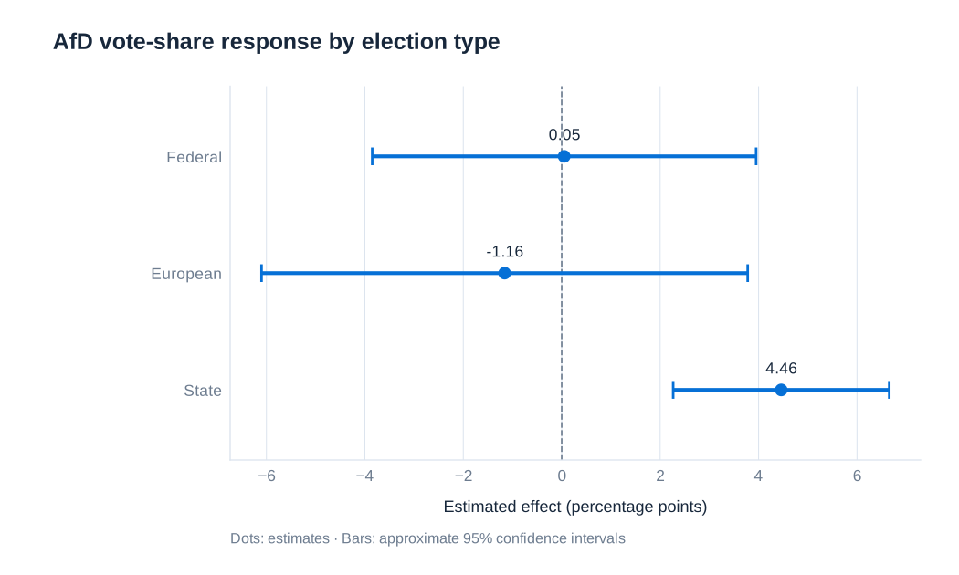
The federal and European estimates are not statistically distinguishable from zero in this baseline. Their uncertainty intervals include effects of both signs, so the evidence does not establish exact zero effects. Likewise, a significant estimate for state elections and an insignificant estimate for another type do not, on their own, constitute a formal test that the two effects differ. That comparison requires the standard error of their difference, including covariance.
The state-election coefficient remains positive across additional specifications: 4.16 points with East-by-year controls, 4.93 when omitting Berlin, 5.87 when removing municipalities with multiple attacks, and 3.34 when including the full set of baseline covariates interacted with year. These are alternative specifications of one substantive question; they should not be averaged as though they were independent studies.
Stress-testing identification and inference
The small failed-only comparison group makes inference a central issue. Hundreds of election observations do not supply hundreds of independent control municipalities. The paper therefore uses wild cluster bootstrap inference, examines the effect of omitting each municipality in turn, and applies an alternative estimator designed for staggered treatment. These checks address uncertainty, influential places and potentially problematic weighting under heterogeneous effects.
A rolling-window analysis includes additional attacks by comparing elections around each municipality–attack episode. This recovers information lost by considering only the first relevant event, but creates another difficulty: an election after one attack can be before a later attack. Overlapping windows make the estimand and dependence structure less simple. The study accordingly treats this as a robustness exercise rather than pretending that every window is an unrelated experiment.
To investigate failed attacks, the researchers construct an alternative comparison group of observably similar municipalities without attacks using propensity-score matching. Successful attacks compared with these matched places produce a state-election estimate of 2.99 percentage points, with a standard error of 1.32. Failed attacks compared with matched places produce −1.69 points, with a standard error of 1.98. The latter estimate is inconclusive. The exercise supports a stronger role for successful attacks but does not establish that failed attacks have precisely zero consequences.
Matching changes the identifying requirement: it relies on the selected observables adequately addressing relevant differences between targeted and untargeted places. It does not manufacture random assignment. Geographic spillovers raise an additional issue because nearby municipalities may respond even without being attacked. The study finds effects in surrounding areas, often about half the baseline magnitude at distances between 25 and 75 kilometres, diminishing by around 80 kilometres. Such responses are informative outcomes in their own right and also warn against assuming that every neighboring municipality is an unaffected control.
Turnout, vote shares and the ecological inference problem
A party can gain votes through newly mobilized voters, switches from other parties, or both. The distinction depends on denominators. Turnout is votes cast divided by eligible voters; a party’s vote share is its votes divided by all valid votes cast. A party-specific participation measure instead divides that party’s votes by eligible voters. These quantities cannot be used interchangeably.
The published estimate for overall turnout in state elections is 0.1469, or 14.69 percentage points. The corresponding AfD-votes-per-eligible-voter estimate is 0.0537, or 5.37 points. Their ratio is approximately 36.6 percent. Describing this as the share of newly mobilized voters choosing the AfD would require assuming no switching between parties. The data show evidence of switching, so the ratio is not an identified individual-level allocation of new voters. It also does not imply that the AfD captured a majority of the turnout increase.
Most major parties receive some additional votes per eligible voter, but the distribution is unequal. The AfD gains a large enough share of the additional support to raise its vote share. The SPD also records a smaller positive state-election vote-share effect, while other major parties show no comparable clear increase. Aggregate results alone cannot reveal precisely which individuals moved from abstention or another party to the AfD. This is the ecological inference problem: changes in group totals do not uniquely identify changes in individual behavior.
Using individual panel data to investigate mechanisms
The German Socio-Economic Panel follows the same people over time and allows the attack data to be linked to their municipality of residence. For an individual , the study estimates:
Person fixed effects remove stable differences between respondents, while year effects absorb common changes. The outcome is an indicator for an attitude or preference, and standard errors remain clustered by municipality because treatment occurs at that level. The regression therefore combines individual-level outcome variation with a group-level treatment design. The following selected estimates are percentage-point changes; the last column gives the number of individuals used for each outcome.
| Individual outcome | Effect, percentage points | Clustered standard error | Individuals |
|---|---|---|---|
| Identifies as right-wing | 6.52 | 2.06 | 2,286 |
| Identifies as hard-right | 4.38 | 1.79 | 2,286 |
| Prefers the AfD | 2.34 | 1.04 | 2,401 |
| Participates in local politics | 2.05 | 0.693 | 3,715 |
| Worried about immigration | 3.61 | 1.74 | 4,102 |
| Worried about terrorism | 0.204 | 2.61 | 2,682 |
The results fit changes in political preferences and participation, not simply changes in the composition of the electorate. However, a stated party preference is not an observed secret ballot, and the different outcomes have different samples and observation frequencies. The small terrorism-concern estimate is especially imprecise. An already high baseline level of concern, around 84 percent, leaves less room for a further increase and may help explain the result without proving a particular psychological mechanism.
Further analysis distinguishes prior partisan attachment from prior political activity. Preference for the AfD increases among some respondents previously attached to the CDU, the Left party and ultra-right parties, as well as among less committed respondents. Previously inactive people also become more likely to prefer the AfD. These findings support both preference switching and political activation; they do not yield a complete, exact accounting of the aggregate vote-share effect. Effects also vary with educational attainment: the shift toward AfD preference is stronger among respondents without a higher-education degree, while the SPD response differs. A genuine heterogeneity claim requires testing the difference between group effects, not simply counting which group has a significant coefficient.
Attack motivation, political messages and media salience
The effects are concentrated in right-wing attacks and attacks directed against foreigners. The published point estimates are about 5.6 percentage points for right-wing attacks and 6.1 for attacks targeting foreigners, compared with smaller and less precise estimates for the alternative categories. These categories can overlap, so they are not additive components of the overall effect. The pattern also does not show that the AfD organized or directed the attacks: electoral benefit and responsibility for violence are different claims.
Political manifestos provide a complementary perspective on how events are framed. The researchers count selected word stems per 10,000 words, subtract a common 2009 CDU manifesto benchmark, and relate those language differences to prior successful attacks at state level. The AfD uses more language connected with crime, naturalization and integration in more exposed states, while responses by other parties differ. The normalization avoids mechanically assigning more occurrences to longer documents, although word counts remain imperfect measures of meaning, emphasis or persuasion.
This analysis has a weaker causal design than the municipality comparison. Aggregating to 16 states reduces independent variation and loses the sharp successful-versus-failed comparison. It therefore supplies evidence consistent with a messaging channel, not a separately randomized estimate of the persuasive effect of those words. Similarly, the media analysis finds more intensive local and regional coverage of successful attacks, with different tone and vocabulary. Highly covered attacks have larger electoral associations, including federal-election effects, but coverage itself is an endogenous response to events. Selection into extensive coverage prevents interpreting that contrast as an experiment that randomly assigns news exposure.
What the case teaches about causal evidence
This application brings several core principles together. A credible comparison is chosen around a plausible source of variation rather than around convenience. The estimand is stated as successful versus failed attacks, with separate evidence needed for attacks versus no attacks. Fixed effects absorb specified forms of heterogeneity, while balance, timing and sensitivity exercises probe remaining threats. Clustered inference respects the level of treatment. Mechanism evidence combines aggregate election outcomes with repeated observations of individuals and political communications, without pretending that these separate analyses fully identify one mediation chain.
The result is historically and institutionally specific: local attacks in Germany over the study period, a particular set of targeted municipalities, and a particular party and electoral structure. It does not establish that every terrorist event in every country benefits the political right. The most useful reading of the study is therefore both substantive and methodological: political violence may change participation and preferences, while the strength of each causal claim depends on its comparison group, identifying assumptions, uncertainty and measurement.
Research source: Navid Sabet, Marius Liebald and Guido Friebel (2025), Terrorism and Voting: The Rise of Right-Wing Populism in Germany, American Economic Journal: Economic Policy, 17(3), 407–440, DOI: 10.1257/pol.20230615. Baseline election results use Table 2; matched-comparison results use Table 3; individual responses use Table 4; partisan and activity analysis uses Table 5. Intervals and percentage-point conversions in this chapter are calculated from the reported estimates and standard errors.