
1. Economic Questions, Data and Causality
This manual develops econometric theory, inference and applications from probability and least squares to modern causal methods, time series, panel data and regularised prediction. The numerical examples and figures are synthetic or schematic teaching illustrations; they are not estimates from an external empirical study.
What econometrics identifies—and what a correlation cannot establish
Economic models and statistical evidence
Econometrics connects economic reasoning to empirical measurement. An economic model proposes mechanisms: demand may respond to prices and income, productivity may respond to schooling, and investments may react to interest rates. An econometric model translates these relationships into observables, unknown parameters and a stochastic disturbance representing influences not explicitly incorporated. The purpose of estimation is not merely to draw a line through data. It is to learn which quantitative statements the available variation can support, with explicit uncertainty and limits of interpretation.
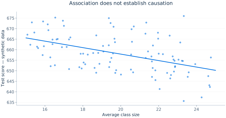
Consider a policy question about school class size. Let Yi denote the average test score of district i, Di its average class size, and Wi observed characteristics such as household income. A useful starting specification is
The outcome Yi and explanatory variable Di are measured, β1 is the parameter of primary interest, Wi′γ summarises measured controls and ui contains omitted determinants and idiosyncratic variation. The slope β1 is a conditional association under the model, unless its identifying assumptions justify interpreting it as a causal effect. If more advantaged districts choose smaller classes, a simple regression may confuse household advantage with school resources. A large sample reduces sampling error, not systematic confounding.
The same distinction applies when an analyst asks whether training raises wages, whether higher cigarette taxes decrease smoking, whether institutions determine income, or whether a yield-curve spread forecasts GDP growth. Forecasting requires useful information about future outcomes; identifying a causal parameter requires credible comparisons between counterfactual outcomes. A variable can be an excellent predictor without producing the outcome it predicts.
Data structures and research designs
Cross-sectional data observe many units at one time, such as household income and education across individuals. The subscript i indexes individuals, firms, districts or countries. A random cross section makes sample averages and regression coefficients natural estimates of population characteristics, although nonresponse, clustering, selection and missingness can invalidate a naive random-sampling model.
Time-series data observe a variable, or several variables, over time. The chronological order matters because Yt can depend on Yt₋1. Trends, changing volatility, seasonal patterns and dynamic responses force us to reconsider assumptions appropriate for independent observations. Time-series data also support genuine forecasting, which must be assessed using observations not used to fit the forecasting model.
Panel or longitudinal data observe the same economic units in several periods and write their outcomes as Yit. A panel can separate persistent differences between individuals from changes occurring within individuals. For instance, differences in managerial ability across firms may contaminate a cross-sectional correlation between capital and profits, whereas repeated observations may make it possible to control for time-invariant ability.
Repeated or pooled cross sections differ from true panel data: samples from different periods need not contain the same people. Each design implies a different sampling model and affects the credible range of empirical questions.
| Data structure | Typical index | Illustration | Main concern |
|---|---|---|---|
| Cross section | i | Firms in 2026 | Selection and confounding |
| Time series | t | Quarterly GDP | Serial dependence and trends |
| Panel | i,t | Same firms 2020–2026 | Unobserved heterogeneity |
| Pooled cross sections | i,t | Different workers in 2020 and 2026 | Composition changes |
Potential outcomes and the selection problem
To formalise a causal question, imagine that each unit has two potential outcomes: Yi(1) if it receives a treatment and Yi(0) if it does not. Let Di ∈ {0,1} indicate the treatment actually received. Only one potential outcome is observed:
The individual causal effect is Yi(1) − Yi(0), but we cannot directly observe both outcomes for a given unit. We often target the average treatment effect ATE = E[Y(1) − Y(0)] or the average treatment effect on the treated ATT = E[Y(1) − Y(0) | D=1]. These are different quantities when treatment effects are heterogeneous and selection depends on the gains from treatment.
An observed difference in group means can be decomposed exactly:
The expression in braces is selection bias: the difference that would exist between treated and untreated groups even if nobody were treated. If intrinsically sicker patients are more likely to receive hospital care, a simple comparison of health outcomes can suggest that hospitals worsen health even when treatment is beneficial. This illustrates why large and statistically precise associations can be causally misleading.
In a well-run randomised controlled trial, treatment assignment is independent of both potential outcomes, and treatment and control groups have identical expected counterfactual outcomes. Consequently their difference in expected observed outcomes identifies the ATE. Random assignment does not guarantee that finite samples balance perfectly, and noncompliance, attrition, interference or measurement problems still require attention.
Estimand, estimator and estimate
The estimand is the precisely defined population quantity of interest, such as the causal effect of reducing class size by one student. An estimator is the random rule applied to data, such as the OLS coefficient calculated from a sample; the estimate is the numerical value obtained when that rule is applied to the observed data. Confusing these concepts leads to overconfident interpretations: a precisely computed estimate need not target the causal effect described in the research question.
Good empirical work specifies the unit of observation, population, measurement convention, parameter of interest, identifying source of variation, plausible competing mechanisms and inference procedure. A standard error measures sampling variation under a model, not the credibility of the identifying assumptions. Identification is conceptual; inference is statistical; neither can replace the other.
Questions for an empirical project
Before computing any regression, ask what intervention or policy change the research seeks to understand, what comparison approximates the ideal experiment, whether the variation in the explanatory variable is plausibly as good as random conditional on controls, and which population the estimated parameter represents. A second set of questions concerns whether standard errors accommodate clustering or serial dependence, whether there are enough independent units and whether the result is practically meaningful.
From a question to a research specification
Imagine an economist asked to estimate how an increase in university tuition influences enrolment. A careless analysis regresses enrolment on tuition and calls the slope a demand elasticity. A disciplined analysis asks first whether tuition varies across institutions, people or time; whether scholarships change net prices; whether students sort into universities because of quality; and whether universities adjust tuition in response to demand. A valid demand elasticity describes changes in choices when the price changes for reasons not themselves caused by shifts in demand. Prices observed at equilibrium may therefore be endogenous.
The target could be a one-percent increase in tuition, a €1,000 level increase or a discrete policy change from one fee schedule to another. Each intervention has different consequences and may not be identified from the same data. For example, if some institutions admit only wealthy applicants, there may be little overlap in the students who face different prices. Estimands should be specified at the relevant margin and for the population directly exposed to that margin.
Economic interpretation also requires accounting for general equilibrium and spillovers. A programme that raises training among some workers may alter wages or job opportunities for untreated workers; in that case their observed outcomes are not unaffected controls. The stable-unit-treatment-value assumption (SUTVA) combines restrictions on interference and the definition of treatment versions. In many economic applications these restrictions are substantive assumptions, not innocuous statistical conventions.
Representative examples of prediction and causal inference
Suppose an analyst uses prior-year sales, website visits and seasonal indicators to forecast next-month sales. This predictive problem concerns accuracy and stability under future conditions. It need not imply that increasing visits through artificial traffic would raise sales. A second analyst studies whether an advertising subsidy causes sales growth. That causal problem requires treatment assignment independent of potential sales outcomes conditional on an appropriate design. Both analysts can use regression, but they answer different questions and may need different covariates and validation procedures.
Another complication is policy response. If local governments increase spending when unemployment begins rising, a cross-sectional or time-series spending coefficient may be positively related to unemployment even if extra public spending partially offsets job losses. A causal effect can have a different sign from its observational association because policy is targeted where outcomes are expected to deteriorate. State what government would have done in the absence of the policy and how that counterfactual can be approximated.
2. Probability for Economic Data
Random variables, joint distributions, conditional expectations and sampling
Random variables and distributions
A random variable assigns a numerical value to each possible outcome of an uncertain process. Discrete random variables possess a probability mass function p(x) = P(X=x), and their probabilities sum to one. Continuous random variables are represented by a density f(x): probabilities correspond to areas under the density, not to its value at a single point. The cumulative distribution function F(x)=P(X≤x) exists for both types and is nondecreasing.
An economic variable often has a skewed distribution: earnings, wealth and firm size can have a long right tail. A sample mean describes average income, while a median can convey the experience of a typical observation more effectively. Neither statistic alone characterises dispersion or the differences between population subgroups.
Expectations, variance and covariance
The expected value is the probability-weighted average of possible outcomes. For a discrete variable it is E[X] = Σx x p(x); in the continuous case E[X] = ∫x f(x)dx, whenever the integral exists. Linearity makes expectations especially useful:
Unlike linearity of expectations, independence is required for some convenient simplifications of variance. The population variance is Var(X)=E[(X−μx)2]=E[X2]−μx2, with standard deviation σx = √Var(X). Variance is measured in squared units; standard deviation returns to the scale of X. For constants a and b, Var(a+bX)=b2Var(X).
Covariance measures signed joint variation:
The correlation coefficient ρx𝓏=Cov(X,Z)/(σxσ𝓏) is dimensionless and lies between −1 and 1. Correlation zero rules out a linear association but not all nonlinear dependence. Independence implies zero covariance when moments exist, but zero covariance does not generally imply independence. For example, if X is symmetric about zero and the required moments exist, X and its square X2 can be uncorrelated while X2 is completely determined by X.
The variance of a sum is
If covariance is negative, combining variables can reduce risk. This is the statistical foundation of portfolio diversification; independent variables have zero covariance, but the useful variance formula does not itself require independence.
Conditional expectations and the law of iterated expectations
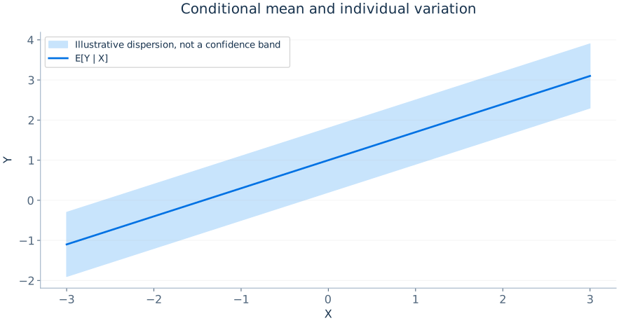
The conditional expectation E[Y|X=x] is the average value of Y among observations with X=x in the population distribution. It is a function of x, not a constant. For the income–consumption relationship, it describes average consumption at different income levels. The conditional expectation function (CEF) is the unrestricted mean relationship, while a linear regression will approximate this relationship using a linear combination of regressors.
The law of iterated expectations states
One can obtain the overall average by first averaging Y within groups defined by X and then averaging those group means using the groups' population probabilities. Define ε=Y−E[Y|X]. By construction E[ε|X]=0, and ε is uncorrelated with every integrable function of X. This exact decomposition does not require that the CEF be linear.
The law of total variance refines this decomposition:
Its first component measures variation in conditional means across X and its second measures average variation within the X groups. This helps explain regression fit as the division between predicted and unexplained variation.
Conditional independence
If Y and D are conditionally independent given X, knowledge of D adds no information about the distribution of Y once X is known. For causal inference, the stronger requirement is often that the vector of potential outcomes (Y(0),Y(1)) be independent of treatment D conditional on pretreatment controls X. This is sometimes called unconfoundedness or selection on observables. It is an assumption about unobserved counterfactuals, not something a high regression R2 can establish.
Conditional independence does not mean that X has no relation to treatment or outcome. Its purpose is to ensure that comparisons within values of X are credible. Overlap, 0<P(D=1|X=x)<1 for the values under study, is also needed to compare treated and untreated units with similar characteristics. If a certain subgroup is always treated, untreated counterfactuals for that subgroup cannot be recovered nonparametrically from the observed sample.
Random sampling and descriptive statistics
Under independent, identically distributed sampling, each observation follows the same population distribution and is independent of the others. The sample mean and unbiased conventional sample variance are
The standard error of the sample mean is σ/√n when σ is known and sampling is independent; s/√n estimates it in ordinary applications. The factor √n is central: quadrupling an independent sample typically halves the standard error. Systematic bias, however, generally does not disappear merely by increasing n.
Probability distributions used in inference
A normally distributed variable is symmetric and completely described by its mean and variance. If Z is standard normal, P(|Z|≤1.96)≈0.95. The χ2 distribution arises from sums of squared standard normal variables. Student's t distribution arises when a normal quantity is divided by an independent estimated standard deviation, with degrees of freedom affecting tail thickness. The F distribution is a ratio of suitably scaled independent χ2 variables and appears in tests of several linear restrictions.
These distributions are important because testing procedures require statements about the sampling behaviour of estimators. Whether an exact t or F distribution is justified depends on stronger assumptions than those needed for a large-sample normal approximation.
Law of large numbers and central limit theorem
The weak law of large numbers (LLN) establishes convergence of a sample average towards the population mean under suitable sampling and moment conditions. The central limit theorem (CLT) characterises the sampling distribution of its deviations. For independent observations with finite variance,
The arrow denotes convergence in distribution. The LLN explains why estimation becomes accurate as n grows; the CLT explains how its uncertainty may be quantified. A normally shaped sampling distribution does not mean that individual wages, earnings or firm profits follow normal distributions.
Bayes' rule and conditioning on events
Bayes' rule is a systematic way to update a probability after receiving information. For events A and B with P(B)>0,
Suppose 4% of firms in a sector will default over the year. A screening indicator is positive for 80% of eventual defaulters and for 15% of non-defaulters. The probability of a positive signal is 0.80×0.04+0.15×0.96=0.176. The probability of default given a positive signal is 0.032/0.176≈0.182, or 18.2%. The signal identifies heightened risk but does not imply an 80% default probability. This distinction illustrates the economic importance of base rates for credit-risk analysis and classification models.
Conditional probabilities extend to continuous variables through conditional densities. For continuous Y and X with a joint density, f(y|x)=f(x,y)/fx(x) wherever fx(x)>0. The conditional mean E[Y|X=x] integrates y over this conditional density. A regression models some aspect of this conditional distribution, not the full joint distribution unless additional statistical assumptions are imposed.
Jensen's inequality, expected utility and log transformations
For a concave function h, Jensen's inequality implies E[h(X)]≤h(E[X]) under appropriate conditions; the inequality reverses for convex functions. Since ln is concave, E[ln Y]≤ln(E[Y]) for positive Y. This explains why the mean of log income is not the log of mean income. It also matters for interpreting estimated log regressions and for the distinction between average proportional changes and changes in an arithmetic average.
In economic decision theory, concavity of utility creates risk aversion: the utility of expected wealth can exceed expected utility of risky wealth. Econometrically, applying transformations to the outcome changes the loss function and the quantity whose conditional expectation the regression approximates. A model of log wages is not simply a numerical convenience equivalent to a model of wages.
The covariance of sample averages under dependence
For independent identical observations, Var(Ȳ)=σ2/n. Without independence, the variance of the average is
The cross-covariance terms vanish under independence, but not for students within the same classroom or repeated observations from one firm. This identity is the elementary reason that clustering and serial correlation affect standard errors. If every student's error includes the same classroom shock, the effective amount of information may be much closer to the number of classrooms than to the total number of students.
3. Statistical Estimation and Inference
Sampling distributions, bias, consistency, efficiency and uncertainty
Parameters and estimators
A parameter is a fixed feature of a population distribution; an estimator is a random variable because it changes across samples. The bias of θ̂ is E[θ̂]−θ, and unbiasedness means its expectation equals the parameter. Consistency means the estimator approaches the parameter in probability as the sample expands; these are not equivalent properties. An estimator can be biased in small samples and still be consistent, or unbiased under particular conditions and yet have unacceptably high variance.
Mean squared error (MSE) combines bias and sampling variance:
A mildly biased estimator can have smaller MSE than an unbiased alternative. This is a major rationale for shrinkage methods in prediction. For causal estimation, however, we must carefully distinguish sampling MSE from identification bias: shrinking a coefficient cannot repair a bad instrument or confounding by unobserved variables.
Sampling distribution of the average
For an independent sample with finite variance σ2, E[Ȳ]=μ and Var(Ȳ)=σ2/n. If the underlying observations are normally distributed, the sample mean is exactly normal for any n. Otherwise it is often approximately normal in sufficiently large samples by the CLT. A sampling distribution is an imagined distribution across repeated datasets drawn by the same mechanism; one normally observes only one dataset and estimates the resulting uncertainty.
The estimated standard error SE(Ȳ)=s/√n is itself random. When errors are normally distributed and σ2 is unknown, (Ȳ−μ)/(s/√n) follows a Student t distribution with n−1 degrees of freedom. The tails approach standard normal as the degrees of freedom increase. Where the normal assumption is implausible, a large-sample normal approximation can remain useful, subject to the CLT and a trustworthy variance estimator.
Confidence intervals
A 95% confidence interval is a random interval procedure whose coverage probability is 95% under the assumed model and repeated sampling. It is not, in classical frequentist terminology, a statement that there is a 95% probability that a fixed realised interval contains the fixed parameter. An approximate interval is
For a small normal sample with unknown variance, the multiplier is usually the appropriate t critical value instead of 1.96. Intervals must use a variance estimator consistent with the data design. Independence-based confidence limits will often be too narrow with positively correlated observations.
Hypothesis testing
A statistical test uses an estimator's sampling distribution to evaluate whether observed evidence is compatible with a null hypothesis. For H0: θ=θ0, the familiar statistic is
A p-value is the null probability of obtaining a test statistic at least as extreme as that observed, as defined by the alternative. It is neither the probability that H0 is true nor the probability that the alternative is correct. A 5% two-sided test rejects for sufficiently extreme positive or negative t values; a one-sided test assigns the rejection region to one tail in advance.
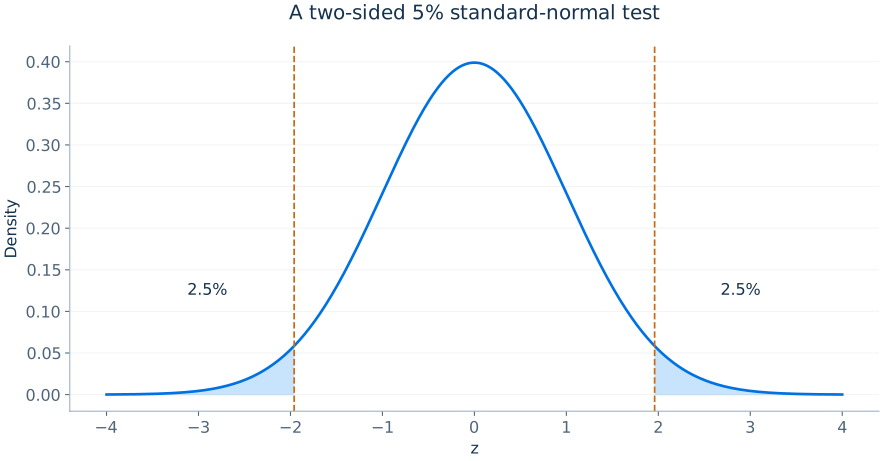
There are at least three distinct standards for discussing an estimate: statistical significance, economic magnitude and identification quality. A coefficient can be statistically distinguishable from zero while too small to matter economically. Conversely, a large estimated policy effect might have a wide confidence interval because the independent sample is small. Neither pattern alone proves causality.
Comparing two population means
For independent samples from groups A and B, the difference in sample means Δ̂=Ȳa−Ȳᵦ estimates the corresponding difference in population means. If the groups are independent, an estimated standard error allowing unequal variances is
Pooling group variances is not necessary unless the equal-variance model is explicitly justified. If the observations instead come in matched pairs or repeated measures on the same units, the covariance between observations changes the variance formula; treating pairs as independent wastes information or understates uncertainty.
Error sources that confidence intervals do not fix
The standard error accounts for sampling variation under the chosen sampling model. It does not automatically account for coding errors, biased measurement, selective publication, misspecified dynamics, omitted confounders or invalid instruments. Confidence intervals quantify one part of uncertainty: they do not certify the validity of the economic interpretation. This separation becomes essential as methods become more sophisticated.
The bootstrap and its correct scope
A nonparametric bootstrap repeatedly samples observations with replacement from the observed empirical distribution, recomputing the estimator for each pseudo-sample. The resulting distribution of bootstrap estimates approximates the estimator's sampling distribution under suitable conditions. Percentile, basic and studentised bootstrap intervals can differ, particularly when distributions are skewed. Bootstrapping should follow the data-generating structure: resample clusters rather than individual students if the statistical units are classrooms, and use appropriate time-series block schemes when observations are serially dependent.
The bootstrap is not a universal solution to identification or weak-instrument problems. Resampling a confounded observational dataset reproduces its confounded association; it does not recreate an ideal experiment. Standard bootstrap procedures can also fail for nonsmooth estimators and nonregular parameters. A resampling method must be validated for the estimator and sampling scheme in use.
Type I and Type II errors
A Type I error is rejection of a true null. For a correctly calibrated 5% test, its probability under the null is 5%. A Type II error is failure to reject a false null; power is one minus the Type II error probability for a specified alternative. These probabilities vary with sample size, population variance, the size of the genuine effect, and the testing design. A 5% significance threshold is not a substantive guarantee that a published claim is likely true.
4. The Simple Linear Regression Model
Deriving OLS and interpreting the slope, intercept, predictions and residuals
Population model and least-squares criterion
The simple linear regression model writes the outcome as a linear function of one explanatory variable and an unobserved disturbance:
The intercept β0 is the conditional mean at X=0 if E[u|X]=0 and X=0 lies in the meaningful range of the data. The slope β1 measures a one-unit change in the conditional mean of Y for a one-unit change in X, conditional on the model. The error term gathers unobserved determinants; it is not simply a synonym for mistakes by the researcher, although mismeasurement can be one of its components.
The ordinary least squares estimator selects b0 and b1 to minimise squared fitted residuals:
Squaring makes negative and positive residuals contribute positively and gives greater weight to larger absolute errors. This criterion is a well-defined sample operation, independent of whether the regressor was randomly assigned. Its causal interpretation is a separate question.
Deriving the slope and intercept
Differentiate the sum of squared residuals with respect to b0 and b1 and set the derivatives equal to zero. The first normal equation states that the sample residuals sum to zero; it implies that the fitted line passes through the sample averages (X̄,Ȳ). Substituting b0=Ȳ−b1X̄ into the second normal equation yields
Thus the slope is the sample covariance divided by the sample variance of X, using the same normalisation in numerator and denominator; equivalently, it is the centred cross-product sum divided by the centred squared-X sum. A flat X with no variation makes the denominator zero: the slope cannot be estimated. The numerator is positive when high-X observations systematically coincide with high-Y observations and negative in the opposite case.
Residuals, fitted values and OLS identities
The fitted value is Ŷi=β̂0+β̂1Xi and the residual is ûi=Yi−Ŷi. With an intercept, OLS normal equations guarantee Σûi=0 and ΣXiûi=0. Consequently the sample covariance between fitted values and residuals is zero, and mean fitted Y equals observed mean Y. These are algebraic properties of the fitted sample, not proof that the unobserved population disturbance is independent of X.
The exact sample variance decomposition is
The three terms are respectively total sum of squares (TSS), explained sum of squares (ESS) and residual sum of squares (RSS, also called SSR in some conventions). It follows that 0≤R2≤1 in an OLS regression containing an intercept, assuming a nonconstant outcome.
Binary regressors: comparing means by regression
Suppose D takes values zero and one and Yi=β0+β1Di+ui. OLS sets β̂0 equal to the observed mean outcome among D=0 and β̂0+β̂1 equal to the mean among D=1, so
A regression with one treatment dummy and an intercept exactly reproduces the difference in sample means. If the treatment was randomly assigned and there is no problematic attrition or interference, it can estimate an average causal treatment effect. If the dummy indicates self-selected college attendance, the coefficient may reflect pre-existing differences in ability or family background.
Rescaling and functional forms
A coefficient depends on units. If X is measured in thousands instead of individual euros, its coefficient increases by a factor of one thousand, while the fitted values and substantive implications remain unchanged. Changing the scale of Y multiplies the coefficient and fitted residuals by the same factor. Transformations must always be interpreted in terms of original economic units.
A level-level model Y=β0+β1X+u has β1 units of Y per unit of X. A log-level model log(Y)=β0+β1X+u has an approximate 100β1-percent change in Y per unit increase in X; the exact proportional effect for a unit change is exp(β1)−1 under appropriate log-scale interpretation. In level-log models the outcome changes by approximately β1/100 units for a 1% change in X. In log-log models β1 is the elasticity of Y with respect to X.
Why an estimated line is not the data-generating process
Regression estimates a best-fitting sample relationship. Even if the population conditional mean is nonlinear, the population least-squares line remains meaningful as the best linear prediction under squared-error loss. If Y is driven by X2, a fitted slope may vary markedly when the observed range of X changes, despite technically correct OLS computation. The fitted line is an approximation; the economic researcher must argue when it is a useful approximation and whether it has an acceptable causal meaning.
The population linear projection
To understand OLS without assuming a truly linear economic mechanism, define the population linear projection as the choice of α and β minimising E[(Y−α−βX)2]. Its slope is β=Cov(X,Y)/Var(X) whenever these moments exist and Var(X)>0. The projection error e=Y−α−βX is orthogonal to the constant and X: E[e]=0 and E[Xe]=0. However E[e|X]=0 need not hold if the true conditional expectation is nonlinear. The difference matters: sample orthogonality is an algebraic result, while conditional mean independence is a richer property of the population distribution.
For a nonlinear conditional expectation, the linear projection is a weighted compromise across observed values of X. The slope can be a useful summary of average linear association and can provide a good forecasting benchmark over the sample's covariate range, even when it should not be interpreted as an invariant structural derivative. The researcher must identify what the coefficient means before attaching a policy interpretation.
Leverage, outliers and influential observations
An observation with an unusual regressor value can have high leverage, meaning it has substantial potential to influence the fitted line. In matrix OLS, leverage hi is the corresponding diagonal element of Px=X(X′X)-1X′. Large residuals and high leverage are distinct properties: an observation can be far from the predictor centre but lie almost exactly on the fitted line; another can have an ordinary X value but an unexpectedly high or low Y.
Influence measures combine leverage and residual size to assess the effect of removing observations. A suspicious record might indicate coding or measurement error, but genuine rare observations may carry essential economic information. Deletion based solely on whether a point weakens statistical significance undermines empirical credibility. Report meaningful changes under sensitivity checks and justify exclusions using defensible data-quality rules.
5. Multiple Regression and Partial Effects
The ceteris paribus interpretation, regression anatomy and multicollinearity
Why multiple regression is necessary
Economic outcomes rarely respond to a single observed determinant. Workers with more education also tend to differ in experience, sector, location and family circumstances. A regression of wages on education alone incorporates all dimensions correlated with education into the same slope. Multiple regression attempts to describe the association of wages with education while holding selected other characteristics fixed. Write
Here each βj describes the change in the conditional linear predictor of Y associated with a one-unit increase in Xj holding the other regressors fixed. This phrase is an interpretation of a mathematical conditional comparison, not a guarantee that such a comparison can be made for the observed population or that βj represents a causal effect.
For example, suppose annual earnings are related to schooling, experience and industry. An education coefficient in this model refers to workers of equal included experience and industry. If ability is unmeasured and affects both schooling and earnings, the education coefficient can still be biased. More variables are not always better: conditioning on mediators of an effect or on colliders may create new biases rather than remove confounding.
How OLS solves the multiple-regression problem
The OLS estimator minimises the sum of squared residuals over all k+1 coefficients. With an n×(k+1) design matrix X, an n-vector y and coefficient vector β, the model and least-squares objective can be written as
Differentiating gives the normal equations X′Xβ̂=X′y. If X has full column rank, the unique solution is
The matrix X′X encodes variation and correlations among regressors; X′y encodes their covariation with Y. Full column rank rules out exact linear dependencies and requires at least as many rows as parameters. Positive residual degrees of freedom additionally require n>k+1; statistical independence is a separate sampling assumption. It is not the same as assuming the explanatory variables are mutually uncorrelated: strongly correlated regressors can be estimated, although with lower precision.
A projection matrix Px = X(X′X)-1X′ satisfies ŷ=Pxy, while residuals are û=(I−Px)y. The projection makes the residual vector orthogonal to every included regressor, X′û=0. These expressions reveal the geometric interpretation of OLS as projection onto the column space of X.
The Frisch–Waugh–Lovell theorem
The Frisch–Waugh–Lovell (FWL) theorem gives an intuitive recipe for understanding β̂1. First regress X1 on all other included explanatory variables and save its residual r1. Second regress Y on those same other variables and save residual rᵧ. Finally regress rᵧ on r1 without an additional intercept. The slope equals β̂1 from the full multiple regression:
The coefficient uses variation in X1 that cannot be linearly predicted by the other regressors. If education is almost perfectly predicted by age and occupational controls, little independent variation remains for identifying its slope. FWL also explains why adding controls can alter an estimate: the relevant variation in X1 is redefined, not simply the number of residual degrees of freedom.
For partialling out it is mathematically valid to residualise Y and X1 on the other controls. It is not generally enough to residualise Y alone, because the denominator and the covariance must correspond to the adjusted variation in X1. The two-residual procedure provides a practical diagnostic and is especially useful in high-dimensional nuisance-adjustment methods.
The omitted-variable bias formula
Suppose the true conditional model includes both X and Z:
If Z is omitted, the population simple-regression slope of Y on X satisfies
This exact population formula isolates two ingredients: the omitted variable must affect the outcome (β2≠0) and correlate with the included regressor (Cov(X,Z)≠0). The sign of the bias is the product of these two signs. If ability increases earnings and is positively related to education, omitting ability tends to bias upward the observed schooling association, although the sign and size of actual ability bias are empirical questions.
The formula has a multiple-regression generalisation: replace X by its residual after projection on other included controls, and measure the covariance between this residual and the omitted variable. A variable unrelated to the regressor after appropriate controls cannot induce conventional omitted-variable bias in its coefficient, even if that omitted variable is important for explaining Y.
The dummy-variable trap and qualitative regressors
Dummy variables encode a categorical characteristic. A model with an intercept and three mutually exclusive industry categories normally includes only two dummies, leaving the third as reference. Including all three creates exact multicollinearity because the intercept is the sum of the three indicators. The omitted reference category is not ignored: it is represented by the intercept, and the included dummy coefficients compare groups with that reference group, conditional on other regressors.
Changing the reference category changes the reported dummy coefficients but not fitted values. For a categorical variable with multiple levels, reporting the estimated mean outcomes or explicit pairwise contrasts can be more illuminating than interpreting arbitrary base-category coefficients individually.
Multicollinearity and precision
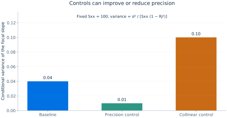
Imperfect multicollinearity means regressors are strongly but not perfectly related. OLS coefficients remain computable, but their variance grows because the residual variation in a particular regressor is limited. Under homoskedasticity,
where Rj2 is obtained by regressing Xj on the other regressors. The variance inflation factor VIFj=1/(1−Rj2) summarises the inflation relative to orthogonal regressors. A large VIF signals reduced precision, not automatically bias or a need to delete economically necessary controls. Whether a variable is appropriate must be decided using the research design.
Scaling, standardisation and interpretation
Standardised variables replace an observed regressor by its deviation from the sample mean divided by its sample standard deviation. If both Y and Xj are standardised, the slope expresses outcome standard deviations per one standard-deviation increase in Xj, holding other regressors fixed. Standardising Xj alone leaves the coefficient in original Y units per standard deviation of Xj. They can facilitate comparisons of association but should not substitute for effects in economically meaningful units. Scaling and centering change intercepts and selected slopes under interactions; they do not create identification.
Consider the fitted model log(wage)=β0+β1educ+β2exper+β3exper2+u. The predicted percentage effect of another year of education is approximately 100β1%, while the marginal change in log wages with respect to experience is β2+2β3exper and varies with experience. Reporting β2 alone as a constant marginal effect is incorrect.
Confounding, precision controls and bad controls
A useful distinction separates controls that protect causal identification from variables that mainly improve precision. A pretreatment variable related to both treatment and outcome can reduce confounding when the conditional-independence assumption is plausible. A baseline variable strongly predictive of outcome but unrelated to random treatment can reduce residual variance and therefore improve precision. A post-treatment variable can instead remove part of the very effect of interest and must not be included automatically. Good modelling chooses controls based on economic timing, institutions and causal logic rather than applying a universal 'include everything' rule.
For example, suppose education affects occupation, which affects wages. When seeking education's total effect, controlling for occupation can block an important causal pathway and produce a different estimand. If occupation is also influenced by unmeasured factors that affect wages, conditioning may create additional bias. A researcher interested in education's direct effect not mediated by occupation requires an alternative estimand and stronger assumptions, not a casual reinterpretation of the same regression coefficient.
Interpreting a full regression table
A carefully interpreted regression table reports coefficient units, explanatory variables, sample size, R2 or comparable fit measure, fixed effects if any and a clear standard-error method. When a coefficient changes after adding controls, several explanations remain possible: omitted confounding in the earlier specification, changes in the analysed sample due to missing control variables, altered weighting implicit in the regression, interactions or functional misspecification. To isolate the effect of controls, compare specifications on a common estimation sample whenever possible.
A policy coefficient can remain nearly constant when controls are added, but coefficient stability alone does not verify exogeneity: all models may omit the same unobserved confounder. Conversely changes across well-justified specifications should trigger substantive inquiry rather than mechanical selection of the coefficient with the smallest p-value.
6. Nonlinearities, Logs and Interactions
Flexible conditional means with coefficients that remain interpretable
Linearity in parameters versus linearity in regressors
The classical least-squares formula estimates models linear in the unknown coefficients, not necessarily linear in the original data variables. A model with X2, log(X), a treatment interaction or year indicators remains linear in parameters if these transformed regressors enter additively with linear coefficients. Conversely Y=exp(β0+β1X)+u is nonlinear in parameters and cannot be estimated as written by ordinary linear least squares without changing the model and error assumptions.
Functional form choices impose substantive statements about marginal effects. Adding a polynomial is not a purely cosmetic technique: it says that the relationship may bend in a systematic way. Using logs can create a proportional-effect interpretation, handle substantial skewness and express economic elasticities. A model must still be checked for sensible predictions, influential observations and any new restrictions imposed by the chosen transformation.
The main logarithmic models
For positive Y and X, four common forms are useful. Level–level: Y=β0+β1X+u has a constant β1-unit marginal change in Y. Log–level: ln(Y)=β0+β1X+u has approximately a 100β1-percent change in Y per unit X. Level–log: Y=β0+β1ln(X)+u has an approximate β1/100-unit change in Y per 1% increase in X. Log–log: ln(Y)=β0+β1ln(X)+u has constant elasticity β1, so a 1% increase in X corresponds to approximately a β1% difference in Y.
| Form | Specification | Coefficient meaning |
|---|---|---|
| Level–level | Y = β0 + β1X + u | Y units per X unit |
| Log–level | ln Y = β0 + β1X + u | ≈ 100β1 % Y per X unit |
| Level–log | Y = β0 + β1ln X + u | ≈ β1/100 Y units per 1% X |
| Log–log | ln Y = β0 + β1ln X + u | Exact elasticity of the exponentiated log predictor: β1 |
When the dependent variable is logged, exponentiating the fitted conditional mean of ln(Y) does not generally reproduce E[Y|X]. Jensen's inequality implies that E[exp(log Y)|X] is not simply exp(E[log Y|X]). Forecasts in original units may require a retransformation or smearing correction, especially with heteroskedastic log residuals.
Quadratic and higher-order terms
A quadratic specification is
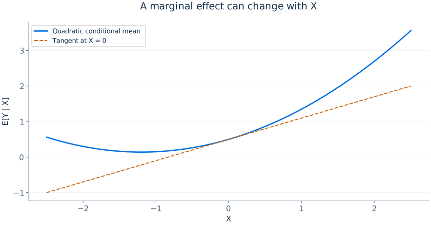
Its marginal effect is β1+2β2X. If β2<0, the function is concave and a positive β1 may eventually turn into a negative marginal effect. The turning point is X*=−β1/(2β2), if β2≠0. One should report whether this point falls inside the observed data range before interpreting it economically. Arbitrarily high-degree polynomials may overfit, fluctuate sharply near boundaries and extrapolate poorly.
Interactions between two continuous regressors
Let E[Y|X,Z]=β0+β1X+β2Z+β3XZ. Holding Z fixed, the marginal effect of X is
The coefficient on X describes its effect at Z=0, which may lie outside the substantively interesting range. Centering Z around its mean makes β1 refer to the average observed level of Z, improving interpretability. The interaction coefficient measures how X's marginal effect changes per unit increase in Z; its sampling uncertainty and the covariance between estimates matter when computing standard errors for a particular marginal effect.
Binary × continuous and binary × binary interactions
The model E[Y|D,X]=β0+β1D+β2X+β3(DX) permits different slopes in treated and untreated groups. For D=0 the slope in X is β2; for D=1 it is β2+β3. The treatment-control contrast at X=x is β1+β3x, not simply β1. The standard error of this contrast uses Var(β̂1)+x2Var(β̂3)+2xCov(β̂1,β̂3).
With two binary variables A and B, adding A×B allows the group possessing both characteristics to differ from the sum of their separate main effects. In a fully interacted model with two binary indicators, fitted means match the four group-specific means. This is an example of a saturated linear model. The same algebra underpins the simplest difference-in-differences specification discussed in the panel-data chapter.
Flexible regression and partial interpretation
A statistical model can flexibly approximate the conditional mean without identifying a causal mechanism. Adding many transformations does not eliminate omitted confounders or endogeneity. An estimated nonlinear regression also requires evaluating the relevant marginal effect at economically appropriate values, accompanied by uncertainty intervals, rather than declaring the coefficient on the original term to be the whole effect.
The multivariate marginal-effect formula
For a smooth conditional mean m(x)=E[Y|X=x], the marginal effect of Xj is ∂m(x)/∂xj. For a discrete or binary treatment, derivatives can be inappropriate; instead calculate the change in predicted outcome between treatment states, holding the remaining covariates fixed. Average marginal effects average unit-specific partial effects across the observed sample; marginal effects at the mean evaluate a nonlinear function at a particular artificial covariate vector. These quantities differ because nonlinear functions do not generally commute with averaging.
If m(X)=β0+β1X+β2X2, the derivative β1+2β2X is individual-specific. The average marginal effect is β1+2β2X̄ in this quadratic case, but more complex functions may require averaging calculated effects over all observations. When models contain multiple interacted covariates, state exactly which are held constant and where the derivative is evaluated.
Inference for turning points and elasticities
The turning point of a quadratic, X*=−β1/(2β2), is a ratio of estimated coefficients. If β2 is imprecisely estimated near zero, this ratio can have a highly skewed distribution; the standard delta method may be unreliable. A graph of the estimated function with confidence bands often communicates uncertainty more responsibly than reporting a single turning-point value. For a predicted effect L(β̂) involving multiple coefficients, incorporate the entire estimated covariance matrix.
Consider a log–log model with estimated slope 0.75 and robust SE 0.12. A simple 95% interval for the elasticity is approximately 0.75±1.96(0.12), or (0.515,0.985). This interval characterises sampling uncertainty in the coefficient under the model, not whether a policy-induced price change has the same effect as a historical market association.
From log predictions to outcomes in original units
A fitted log model describes m(x)=E[ln(Y)|X=x]. Its exponent exp(m(x)) is a conditional geometric mean, and is a conditional median when the log disturbance has conditional median zero. To obtain the conditional arithmetic mean, write Y=exp(m(X))exp(u) and average the second factor conditional on X. The resulting correction can vary across covariate values; exponentiation alone generally understates the conditional mean.
If u conditional on X is normal with constant variance σ2, the correction is exp(σ2/2). With a constant error distribution but without normality, a smearing estimate uses the sample mean of exp(ûi). A single global smearing factor is generally insufficient when the distribution of u changes with X. For example, if m(x)=2 and σ2=0.25, exp(2) is about 7.39 but the conditional mean is exp(2.125), about 8.37. Multiplicative comparisons between two covariate values cancel the correction only if it is identical at those values.
Binary outcomes: linear probability, logit and probit
For a binary outcome, the conditional mean is a probability. A linear probability model uses p(x)=x′β and interprets a coefficient of 0.04 as a four-percentage-point change, holding other regressors fixed. The model is simple but can predict below zero or above one, and its error variance p(x)[1−p(x)] is generally heterogeneous.
Logit uses the logistic distribution function Λ and probit uses the standard normal distribution function Φ. Both keep fitted probabilities between zero and one. With independent observations, maximum likelihood chooses coefficients to maximise the Bernoulli log-likelihood shown below, where pi is the fitted probability and yi is zero or one. A logit coefficient describes a change in log odds, not a percentage-point change. For an untransformed continuous regressor without interactions, its probability marginal effect is βjpi(1−pi); the probit analogue is βjφ(xi′β), where φ is the standard normal density. For binary regressors, compare predicted probabilities at zero and one and average these differences if the estimand is an average effect. These models still require a credible identification argument for causal claims.
| Model | Probability function | Main interpretation |
|---|---|---|
| Linear probability | x′β | Slope in probability units; use a suitable robust covariance |
| Logit | Λ(x′β) | Slope in log odds; calculate probability contrasts |
| Probit | Φ(x′β) | Slope on the normal index; calculate probability contrasts |
7. Finite-Sample OLS Theory
Unbiasedness, conditional variances, Gauss–Markov and normal inference
What finite-sample theory asks
Finite-sample theory characterises estimators for a given n under precisely stated assumptions. It differs from asymptotic theory, which studies sequences of growing samples. In the familiar multiple regression y=Xβ+u, exact statements often condition on the observed matrix X. This is convenient for separating the stochastic properties of the disturbance from the realised variation in the regressors.
The core assumptions are a model linear in coefficients, a sampling mechanism with appropriate independence, no perfect multicollinearity and a zero conditional mean E[u|X]=0. The last assumption is the key to OLS unbiasedness; homoskedasticity and normally distributed disturbances are not needed for unbiasedness. However, unconditional mean zero E[u]=0 by itself is not sufficient because the error could systematically vary with the regressors.
Deriving conditional unbiasedness
Substituting y=Xβ+u into the OLS formula yields
If X has full column rank and E[u|X]=0, conditional expectation immediately gives E[β̂|X]=β. Taking expectations again proves E[β̂]=β. This proof is useful because it displays exactly where exogeneity enters: if E[u|X]≠0, OLS generally contains a systematic component dependent on regressors. Merely estimating a regression does not establish the assumption used to justify its result.
The conditional expectation assumption may fail when omitted variables correlate with explanatory variables, when economic agents jointly determine explanatory and outcome variables, or when a regressor is systematically measured with error. A regression can still compute the coefficient, but its expected value need not equal the structural parameter of interest.
Conditional covariance matrix of OLS
Allow the conditional covariance of the disturbance vector to be Ω=Var(u|X). Direct substitution gives
Under conditional homoskedasticity and no correlation across units, Ω=σ2I; the expression becomes
The ordinary estimated error variance is s2=RSS/(n−k−1) when the model has k explanatory regressors and an intercept. The denominator adjusts for the number of estimated parameters. Under the classical conditional assumptions, it is an unbiased estimator of σ2. Usual standard errors take square roots of diagonal entries of s2(X′X)-1.
If the error variance differs across observations, these conventional standard errors can be inconsistent even when zero conditional mean ensures OLS is unbiased. Robust estimators are addressed separately because changing the variance calculation does not change the underlying estimated slope.
The Gauss–Markov theorem
Under the linear model, full rank, exogeneity and spherical errors (homoskedastic and uncorrelated disturbances), OLS is best linear unbiased (BLUE). "Best" means it has the smallest conditional covariance matrix among linear estimators unbiased for every value of β under the model; it does not mean OLS has the lowest variance among all imaginable nonlinear or biased estimators, nor does it require the disturbances to be normally distributed.
For intuition, consider any other unbiased estimator linear in y: β̃=Ay. Since unbiasedness requires AX=I, write A=(X′X)-1X′+C with CX=0. Under Ω=σ2I, the difference between the competitors' covariance matrices is
Because CC′ is positive semidefinite, no linear unbiased competitor improves on OLS in the positive-semidefinite sense. The proof identifies exactly which assumptions deliver efficiency and why it may fail under heteroskedasticity or autocorrelation.
Sampling distributions under normal disturbances
If u|X is jointly normal N(0,σ2I), then β̂|X is normal with mean β and covariance σ2(X′X)-1. Under this classical normal model, each t-statistic based on an appropriately estimated variance has an exact Student t distribution with n−k−1 degrees of freedom. For q linear restrictions, an appropriately constructed ratio of restricted versus unrestricted sums of squares follows an exact F distribution with q and n−k−1 degrees of freedom.
Without the normality assumption, OLS may remain unbiased and BLUE, while the conventional finite-sample t and F reference distributions are no longer exact. Researchers then commonly rely on asymptotic results and robust standard errors, or carefully justified resampling procedures.
Heteroskedasticity and finite-sample consequences
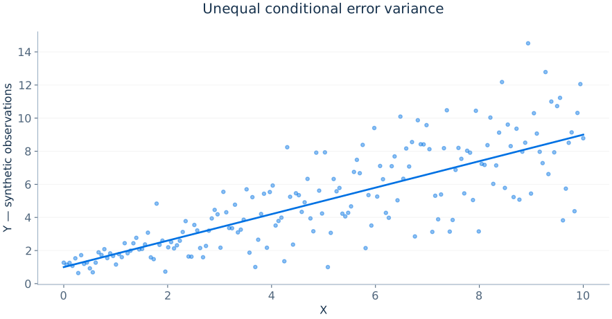
Heteroskedasticity means Var(ui|Xi) changes with the regressors or other information. If E[ui|Xi]=0 remains valid, coefficient unbiasedness can survive; the conventional variance simplification generally cannot. Homoskedasticity tests can sometimes describe variance patterns but are not necessary to justify using heteroskedasticity-robust covariance estimates. Robust standard errors must still be based on a correct independence, clustering or dependence structure.
Gauss–Markov assumptions in plain economic language
The linearity assumption concerns the parametrisation of the outcome's conditional mean, not the absence of nonlinear transformations of observed variables. Random sampling is a description of how economic units enter the dataset. No perfect collinearity requires variation in regressors that cannot be represented exactly by other included regressors. Zero conditional mean states that the excluded determinants do not change systematically with included regressors. Homoskedasticity states that, conditional on the regressors, the unexplained outcome variance is constant; no serial correlation requires distinct disturbances to be uncorrelated. Each assumption must be evaluated in the context of how the data were generated.
The Gauss–Markov claim concerns a particular benchmark class of estimators; it is not a universal claim that simple OLS dominates every alternative. With a known nonspherical covariance Ω, the generalised least squares estimator β̂ᴳᴸˢ=(X′Ω-1X)-1X′Ω-1y may be more efficient when the model and covariance are correctly specified. Feasible GLS estimates Ω from data and therefore introduces additional sampling assumptions and potential sensitivity to covariance-model misspecification.
Homoskedasticity as a special case
For a binary outcome Y taking values zero and one, E[Y|X]=p(X) and Var(Y|X)=p(X)(1−p(X)). Unless p(X) is constant or takes special values, this conditional variance changes with X. A linear probability model therefore naturally exhibits heteroskedasticity even when the mean relationship is correctly approximated. This is a clear illustration of why robust standard errors are not an obscure remedy for rare statistical pathologies; heteroskedasticity often follows directly from the economic data structure.
Weighted least squares and what the weights mean
When the conditional variance is known to be proportional to a positive function hi, dividing each observation’s equation, including the intercept, by √hi makes the transformed disturbance homoskedastic. Weighted least squares therefore minimises squared residuals with weights wi=1/hi. A noisier observation receives less weight because it supplies less information about a common conditional-mean coefficient. W is the diagonal matrix of these positive weights.
Correct variance weights can improve efficiency under the maintained zero-conditional-mean model. Estimated weights give feasible WLS and require checking the variance specification; use a covariance estimator appropriate to the transformed estimating equations when that specification may be wrong. Precision weights are different from survey sampling weights or inverse-propensity weights, which address population representation or causal comparisons. In R, lm(y ~ x, weights = w, data = dat) expects inverse-variance weights for this precision interpretation. When the linear mean is only an approximation, weighting can change the population projection being estimated, so coefficient changes are not automatically evidence of improved causal identification.
8. Analysis of Variance and Model Fit
ANOVA, R-squared, residual diagnostics and predictive accuracy
Orthogonality and decomposition of sums of squares
OLS separates observed outcomes into fitted values and residuals: Yi=Ŷi+ûi. With an intercept, sample orthogonality implies that the total sum of squared deviations from Ȳ is the sum of the squared fitted deviations and squared residuals:
Dividing by TSS gives R2=ESS/TSS=1−RSS/TSS. A value near one means the linear predictors explain much of the sample variation in Y around its sample mean. It does not demonstrate an unbiased causal effect; time trends, common shocks and mechanically related variables can generate very high R2 values without a credible structural interpretation.
The meaning of adjusted R-squared
Adding a regressor cannot increase the in-sample RSS when OLS is recomputed, so ordinary R2 never decreases in nested models. Adjusted R2 penalises the number of estimated parameters:
The adjustment can fall when the added variable improves fit only slightly. It is not an unbiased estimate of out-of-sample prediction quality, and it is not a causal variable-selection rule. Comparisons between models using different dependent-variable transformations require particular caution: R2 values for Y and ln(Y) are not directly comparable measures of fit on the same outcome scale.
Standard error of regression and forecast errors
The residual standard error is SER=√(RSS/(n−k−1)). It estimates the scale of errors in units of Y under relevant assumptions. A predictive application cares about error on data not used to estimate the model. If the fitted model is evaluated on an independent validation sample, a common performance metric is mean squared prediction error:
Root MSPE has the units of the predicted variable and is more interpretable than raw squared errors. For forecasting, validation observations must lie later in time than training observations; randomly shuffling a time series can leak future information into the model-building process.
Residual plots and specification checks
Residual plots against fitted values, each regressor, time and group indicators can reveal outliers, heteroskedasticity, nonlinearity and serial patterns. A residual scatter that fans out suggests a variance model that depends on X. A curved residual pattern suggests omitted nonlinear terms. Serial runs of positive and negative residuals in time-series data suggest dynamic misspecification or correlated disturbances.
However, OLS residuals are orthogonal to included regressors by construction. A zero sample residual–regressor covariance therefore does not validate the zero-conditional-mean assumption. Specification tests are useful diagnostics but cannot by themselves identify unobserved counterfactuals or prove exogeneity.
Overfitting and out-of-sample validation
When the number of regressors becomes large relative to the number of observations, in-sample fit can improve even if the model loses predictive reliability. With n parameters and n observations, it may be possible to interpolate the dataset perfectly, leaving no honest out-of-sample guarantee. Cross-validation, independent test sets and regularisation target predictive performance rather than merely the fitted-data RSS.
| Statistic | What it measures | What it does not prove |
|---|---|---|
| R2 | In-sample variation explained by projection | Causal identification |
| Adjusted R2 | Fit penalised for model size | Best prediction on new data |
| SER | Residual scale in outcome units | No specification bias |
| Out-of-sample RMSE | Typical forecast error in outcome units | Structural effect |
| t-statistic | Signal relative to a specified SE | Economic importance |
Variance in regression output
Statistical software often reports an analysis-of-variance table with model sum of squares, residual sum of squares, their degrees of freedom and the corresponding mean squares. When all conventional homoskedastic assumptions hold, the ratio of model and residual mean squares can provide an overall F-test. With heteroskedasticity, a robust Wald test should replace the conventional sum-of-squares comparison for general joint hypotheses.
Sample fit, causal validity and spurious precision
Three models can report identical R2 values while offering very different information. A randomised treatment regression with a low R2 can identify a credible policy effect, because treatment may explain only a small fraction of individual outcome variation. A high-dimensional prediction model with high cross-validated accuracy may provide excellent forecasts without identifying any causal intervention. A trending time-series regression between unrelated integrated variables may have extremely high R2 while standard t-based inference is invalid. Evaluating these models with one fit statistic is a category error.
Decomposing explanatory contributions
In multiple regression, explanatory contributions of correlated regressors cannot always be separated uniquely. If schooling and parental income are correlated, attributing explained wage variation to each variable depends on the decomposition procedure or order of inclusion. A partial R2 for a selected regressor group measures its incremental fit conditional on the remaining regressors; it should not be interpreted as a unique causal share of the outcome.
Partial R2 can be defined through restricted and unrestricted residual sums of squares: R2partial=(RSSrestricted−RSSunrestricted)/RSSrestricted. The numerator measures the fit improvement from adding the selected regressors, while the denominator is the unexplained variation in the restricted model. It can be useful for assessing a conditional relationship or a first stage, but does not validate the exclusion restriction of an instrument.
Confidence intervals for a mean and prediction intervals for a person
An interval for the conditional mean answers how precisely average Y at x0 has been estimated. A prediction interval asks where a new individual outcome Y0 may fall. The second interval includes both uncertainty about the estimated mean and the new observation’s irreducible disturbance, so it is wider under the same model. Here x0 includes the intercept, s2 is the conventional residual variance estimate, p is the total number of fitted coefficients and h0=x0′(X′X)-1x0.
Under the correct homoskedastic normal linear model and an independent new observation, the two intervals use the formulas below. The extra 1 inside the prediction square root is the new disturbance variance in units of s2. Even with a huge estimation sample, this uncertainty does not disappear. Leverage makes both intervals wider away from well-supported covariate values. R distinguishes interval="confidence" from interval="prediction" in predict.lm. Robust coefficient standard errors alone do not construct a valid heteroskedastic prediction interval: the conditional distribution of the new outcome also needs attention.
9. Hypothesis Tests in Regression
t-tests, confidence intervals, F-tests, Wald tests and joint restrictions
A general approach to hypothesis testing
Testing starts with a population-level hypothesis. The null may claim that education has zero conditional association with wages, that a policy affects neither employment nor investment, or that two groups have the same regression slope. The hypothesis must be stated before interpreting results so that the number of restrictions, relevant estimators and reference distribution can be chosen appropriately.
For a single linear coefficient, H0: βj=βj,0, the usual test statistic is
When the standard error consistently estimates sampling uncertainty, t is often approximately N(0,1) under the null in large samples. Exact Student t inference additionally requires the relevant normal and classical linear-model assumptions. The p-value measures how surprising the observed statistic would be if the null and its sampling assumptions were true.
Confidence intervals and the link with two-sided tests
An approximate 100(1−α)% interval for βj is β̂j ± z1₋α/2 SE(β̂j). At the 5% level, the two-sided test H0:βj=0 rejects exactly when zero is outside its corresponding two-sided 95% interval, provided both use the same SE and critical distribution. The interval displays the range of parameter values not rejected by the corresponding procedure and provides more information about possible economic magnitudes than a binary significant/nonsignificant statement.
Joint restrictions and why separate t-tests are insufficient
A model may contain a quadratic polynomial or a set of industry indicators whose joint effect is of interest. Testing each coefficient individually at 5% does not test the set of null restrictions at a 5% family level. The appropriate joint null can be written
where R is a q×(k+1) matrix identifying the q restrictions and r is a q-vector of hypothesised values. A general Wald statistic measures how far Rβ̂ is from r relative to the joint covariance of the estimates:
For asymptotic tests, W converges to a χ2 distribution with q degrees of freedom when the null holds and suitable regularity assumptions apply. Many packages report F=W/q and use an appropriate reference distribution. A heteroskedasticity-robust V̂ should be used when constant error variance is not justified.
The restricted versus unrestricted F-test
Under the classical normal homoskedastic model, one can compare a restricted regression satisfying the null to an unrestricted regression that includes all parameters. The standard partial-F statistic is
Restrictions cannot reduce the minimal RSS, so RSSr≥RSSu. The numerator quantifies deterioration in fit per imposed restriction; the denominator estimates disturbance variance from the unrestricted model. Under the null hypothesis and the classical normal, spherical-error assumptions, F follows the central F distribution with q and n−k−1 degrees of freedom. Under a false restriction it generally has a noncentral F distribution. This convenient RSS formula is not generally heteroskedasticity-robust; use the robust Wald formulation when necessary.
A joint F-test on two coefficients can reject even when neither individual t-test rejects, because the estimates' covariance matters. Conversely several isolated significant t-tests are not automatically evidence against a carefully defined joint restriction after accounting for multiple comparisons.
Tests of linear combinations and interactions
Suppose Y=β0+β1D+β2X+β3DX+u. The treatment contrast at X=x is L=β1+xβ3. Its estimate is L̂=β̂1+xβ̂3 and its variance is
Ignoring the covariance term can materially distort the standard error. The same principle applies to sums of coefficients representing total dynamic effects, post-policy effects and returns at a specific value of a moderating variable.
Multiple testing and substantive interpretation
When researchers examine many outcomes, control sets or subgroups and report only the most significant results, nominal p-values can seriously overstate evidence. Adjusting familywise error rates by Bonferroni or using false-discovery-rate procedures may be appropriate for multiple exploratory tests. More generally, transparent research design, reporting complete specifications and distinguishing preregistered confirmatory analysis from exploratory analysis reduces misleading claims.
Power, statistical significance and scale
Statistical power is the probability of rejecting the null for a specified alternative. Larger independent samples and lower noise increase power for a fixed effect, whereas high regressor collinearity, limited treatment variation and correlated errors can reduce it. An insignificant estimate does not prove an effect is exactly zero; it may reveal limited information. A very narrow interval around a small effect can demonstrate that large effects are implausible, which may be more useful than a binary test decision.
A systematic derivation of the partial F statistic
Let the unrestricted model estimate k slope coefficients and an intercept, with unrestricted residual sum of squares RSSu. Imposing q independent linear restrictions produces RSSr, with RSSr≥RSSu because the restricted candidate set is smaller. Under the null restrictions and the spherical normal model, the extra sum of squares divided by σ2 is central χ2 with q degrees of freedom, independent of RSSu/σ2, which is χ2 with n−k−1 degrees of freedom. The ratio of these mean squares therefore has an F(q,n−k−1) distribution. Normality and spherical errors support the exact reference distribution and independence of these quadratic forms. The sample identity TSS=ESS+RSS follows instead from OLS orthogonality with an intercept and needs neither homoskedasticity nor stochastic independence.
The robust Wald test instead uses the estimated covariance of Rβ̂. This generalises beyond the classical covariance formula and allows tests whose restrictions mix several coefficients. A practical R model comparison can report both classical ANOVA and robust Wald results, but the scientifically appropriate one depends on whether the conventional variance assumptions are defensible.
Misreading a nonsignificant coefficient
Suppose a minimum-wage effect on employment is estimated at −0.5% with an approximate 95% interval from −7% to +6%. Calling the result “no effect” is not justified: the data may be compatible with both economically important employment losses and gains. If the corresponding interval were (−0.7%,−0.3%), the effect would be more precisely estimated but perhaps economically small. The width and substantive range of a confidence interval frequently provide more policy information than its relation to an arbitrary zero threshold.
10. Double Selection and High-Dimensional Controls
Post-Lasso inference for a treatment coefficient with many candidate controls
The problem that motivates double selection
Standard low-dimensional regression works when the set of meaningful controls is modest compared with the sample size and the researcher can prespecify a credible adjustment set. Contemporary economic datasets may contain hundreds or thousands of candidate controls, transformations and interactions. If the number of regressors is large relative to n, ordinary least squares can be unstable or impossible to estimate with a unique solution. Purely predictive variable selection is tempting, but selecting controls only because they predict the outcome can jeopardise inference on the treatment effect.
The central model is a partially linear relationship
where D is a treatment or focal regressor, X contains potentially many pretreatment controls and g0 is a high-dimensional nuisance function. The parameter α0 is the target. An auxiliary treatment equation relates D to controls:
The second relationship matters because some controls may be weak predictors of Y but strong predictors of D. Omitting such variables from the outcome model can bias the treatment coefficient when the omitted variables also affect Y.
Why outcome-only selection can be misleading
Imagine Xj has a modest association with test scores but a very strong association with district class size. Selecting variables by their power to predict test scores alone may discard Xj, although it is a confounder relevant to the treatment assignment process. Conversely, selecting only by predictors of D may ignore major determinants of Y that help improve precision. A high-dimensional procedure should protect against both problems instead of treating predictive accuracy in one equation as sufficient.
In a low-dimensional model, the classical omitted-variable bias formula warns that leaving out a confounder requires both a link to D and a link to Y. Double selection addresses this dual requirement systematically by selecting controls from both relationships.
Lasso as a screening device
The Lasso minimises squared errors plus an L1 penalty on regression coefficients:
The tuning parameter λ controls the degree of shrinkage. Because the absolute-value penalty creates corners, coefficients of some predictors can be set exactly to zero, generating a selected set of controls. Standardising predictors before penalisation is usually necessary so that coefficient penalties are comparable. The treatment D is not penalised in the final causal parameter regression; it is the variable whose effect we seek to estimate.
The double-selection algorithm
In a standard partially linear implementation, first run Lasso of Y on the controls X and collect the controls selected for outcome prediction, Sᵧ. Second run Lasso of D on X and collect the controls selected for treatment prediction, Sᴅ. Form their union, S=Sᵧ∪Sᴅ, and estimate an ordinary linear regression of Y on D and all controls in S. The coefficient on D is the post-double-selection estimator of α0.
The union is essential: selecting by either equation alone omits a class of potential confounders. The method is particularly meaningful when there is an approximately sparse representation of the nuisance relationships, appropriate regularity conditions, and a sufficient effective sample size. It does not overcome endogenous D caused by genuinely unobserved confounders; it can only adjust for information represented among the candidate controls.
Orthogonalisation and the double-machine-learning connection
A related technique residualises the outcome and treatment on X and regresses one residual on the other. Let mᵧ(X)=E[Y|X] and mᴅ(X)=E[D|X]. Define residuals Ỹ=Y−mᵧ(X) and D̃=D−mᴅ(X). Under the partially linear model, α0 can be estimated using the moment equation
This moment is Neyman-orthogonal with respect to suitably defined nuisance perturbations: small errors in estimating the nuisance functions have no first-order effect on the target moment at the truth. Cross-fitting—estimating nuisance functions on folds not used for the corresponding residual-based target regression—reduces overfitting bias and is especially important with flexible learners. Double selection and partialling-out double machine learning share an identification framework, but their algorithms and regularity conditions should not be casually conflated.
Conditions, inference and limitations
Post-selection confidence intervals cannot generally be constructed by pretending that a naive single-equation variable-selection step did not take place. Valid double-selection results require assumptions on approximate sparsity, penalty selection, regressor moments, restricted eigenvalues or related design conditions, and suitable rates for nuisance estimation. The exact theorem depends on the estimator and the sample design. Robust or clustered inference must accommodate the actual dependence structure.
If X contains variables caused by D, conditioning on them may remove part of the causal effect or induce collider bias. Thus even a mathematically sophisticated selection algorithm does not choose a causal graph for the researcher. The controls' economic and temporal meaning remains indispensable.
Practical implementation in R
The following code is a schematic implementation for a complete-case dataset containing y, d and numeric controls x1 to x5. All variables must use the same retained rows before model.matrix and cv.glmnet are called. It uses a penalty chosen by cross-validation for illustration; the displayed summary is a software check, not a validated post-selection inference procedure. Published inferential implementations may use theoretically motivated penalty loadings, cross-fitting or dedicated double-selection packages.
library(glmnet)
X <- model.matrix(~ x1 + x2 + x3 + x4 + x5 - 1, data = dat)
fit_y <- cv.glmnet(X, dat$y, alpha = 1)
fit_d <- cv.glmnet(X, dat$d, alpha = 1)
sel_y <- which(as.vector(coef(fit_y, s = "lambda.min"))[-1] != 0)
sel_d <- which(as.vector(coef(fit_d, s = "lambda.min"))[-1] != 0)
keep <- sort(unique(c(sel_y, sel_d)))
final <- if (length(keep) == 0L) lm(dat$y ~ dat$d) else lm(dat$y ~ dat$d + X[, keep, drop = FALSE])
summary(final)
For production work, verify variable mapping and intercept handling, inspect model selection stability, use appropriate heteroskedasticity-robust or clustered standard errors, and consult an inferentially validated implementation rather than assuming the illustrative code constitutes a proof of asymptotic coverage.
Double selection compared with ordinary stepwise regression
Traditional stepwise regression selects variables through sequential significance tests or fit criteria. The procedure often neglects the special inferential status of the focal treatment coefficient and can produce unstable selected models with invalid naive post-selection p-values. Double selection instead builds on the omitted-confounder logic: include controls that predict the outcome or treatment and then estimate the target parameter after taking the union of the selected adjustment variables.
It does not follow that every variable chosen by a machine-learning algorithm is a valid pretreatment control. Economic theory and the temporal ordering of events determine which features can be candidates. If a firm responds to a subsidy by increasing employment and wages, post-subsidy employment should not automatically be controlled for when measuring the subsidy’s total effect on wages, even if an algorithm deems it a powerful predictor.
When sample splitting is useful
In double machine learning, dividing the sample into folds prevents nuisance predictions for observation i from being estimated using that observation's outcome. Each fold's treatment and outcome residuals are constructed with nuisance models trained on other folds. The resulting orthogonal moment reduces first-order sensitivity to regularisation bias under suitable convergence rates. Cross-fitting can improve robustness to overfitting but cannot overcome a failure of conditional ignorability or the absence of overlap.
If the treatment is continuous, the conditional expectation mᴅ(X) is a regression function; for binary treatment it is the propensity score. The same residualisation logic leads to a partialling-out estimator, but the modelling strategy and inference must match the treatment type and statistical design.
11. Large-Sample OLS and Robust Inference
Consistency, asymptotic normality and heteroskedasticity-consistent covariance
Why large-sample theory matters
Finite-sample unbiasedness is attractive but can rely on strong assumptions or may be difficult to establish in complex models. Asymptotic theory instead asks how the distribution of an estimator behaves as the number of appropriately sampled observations grows. Consistency means convergence in probability to the parameter; asymptotic normality characterises fluctuations around that limit on the √n scale. These properties are logically distinct: an estimator can converge to a wrong pseudo-true parameter and still have a normal limiting distribution around it.
In the multiple-regression setting, the OLS identity is β̂=β+(X′X)-1X′u. Reorganising yields
If (1/n)X′X converges in probability to a finite nonsingular matrix Q=E[XiXi′] and (1/n)X′u converges to zero, then β̂ converges to β. The key condition is an orthogonality moment, E[Xiui]=0; conditional mean independence is a sufficient but stronger requirement in standard models.
Deriving consistency
The LLN makes sample averages approach their population counterparts. For identically distributed independent observations, suitable finite moments and nonsingularity imply
Thus E[Xu]=0 gives consistency, while E[Xu]≠0 typically produces a nonzero asymptotic bias. This expression connects large-sample estimation directly to the omitted-variable and endogeneity problems introduced earlier. A sample of one million observations can estimate the wrong population slope with exceptional precision if E[Xu] is not zero.
The asymptotic distribution and the sandwich variance
Let Ω=E[XiXi′ui2]. Under independent observations, appropriate moment conditions and a CLT,
This is the general heteroskedasticity-robust asymptotic covariance formula for a correctly targeted linear moment estimator. The corresponding approximate finite-sample covariance is (1/n)Q-1ΩQ-1. In practice, replace Q and Ω by sample analogues and ui by estimated residuals:
The superscript HC0 labels the basic Eicker–Huber–White form. HC1 multiplies it by an appropriate degrees-of-freedom adjustment, whereas HC2 and HC3 apply leverage corrections observation by observation. The preferred choice can matter with influential observations and smaller datasets.
Why robust standard errors do not fix biased coefficients
Ordinary OLS and heteroskedasticity-robust OLS use the same fitted coefficients. The robust procedure modifies the estimated variance of the estimator, not the identification strategy. If education correlates with omitted ability, calculating HC3 standard errors does not turn the schooling association into a causal return. Inference can be robust to heteroskedasticity while the point estimate remains inconsistent because of endogeneity.
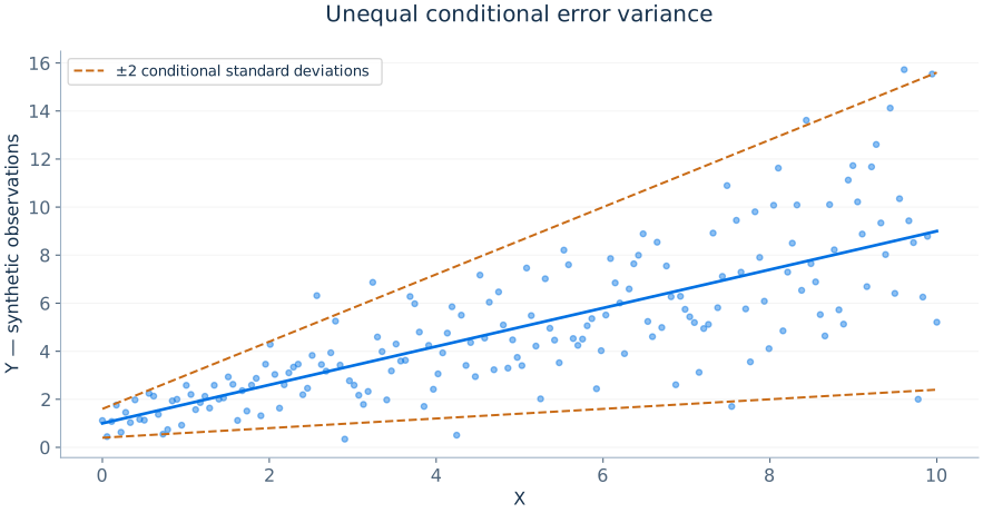
Clustered and time-dependent observations
If students share classrooms, workers share firms or observations are repeated within countries, errors may be correlated within clusters. Treating clustered observations as independent can produce severe overconfidence. Cluster-robust covariance estimators aggregate score contributions within each independent cluster; the effective amount of information often depends more on the number of independent clusters than on the raw count of observations.
Let Xg and ûg contain observations from cluster g. An uncorrected cluster sandwich has the form
Practical procedures apply small-sample corrections and use cluster-aware reference distributions. With very few clusters, standard asymptotics may be unreliable; appropriate cluster-specific bootstrap methods or alternative research designs may be necessary. For time-series data, heteroskedasticity-and-autocorrelation-consistent (HAC) covariance estimation explicitly accounts for correlation across lags.
The delta method for nonlinear quantities
Economists often report a function g(β̂), such as an elasticity, a ratio of coefficients, a turning point or a cumulative dynamic effect. If β̂ is asymptotically normal and g is differentiable at the target, the delta method gives
For a ratio g(a,b)=a/b, the gradient is (1/b, −a/b2). Ratios become unstable when the denominator is near zero, so first-order delta approximations may perform poorly—an important warning for instrumental-variable estimators with weak first stages.
Practical robust testing
Use a robust covariance estimator consistent with the observational design, not simply a default option. HC standard errors assume independence across observations (though they permit unequal error variances), while cluster and HAC estimators target different dependence structures. The relevant regression output should disclose the number of observations, controls, cluster units and standard-error estimator.
fit <- lm(y ~ x1 + x2 + x3, data = dat)
library(sandwich)
library(lmtest)
coeftest(fit, vcov. = vcovHC(fit, type = "HC3"))
# Cluster-robust inference when 'firm_id' identifies independent firms:
coeftest(fit, vcov. = vcovCL(fit, cluster = ~ firm_id))Robust variance and the hat matrix
The leverage of observation i in linear regression is hi=xi′(X′X)-1xi. In small samples, fitted residuals can systematically understate disturbances at high-leverage observations. HC2 replaces ûi2 by ûi2/(1−hi), while HC3 uses ûi2/(1−hi)2 inside the sandwich “meat”. These corrections can produce materially different standard errors where the design contains unusual X values.
No HC estimator repairs cross-observation dependence. For example, if 500 students come from 10 classrooms, an HC3 calculation still treats the rows as independent. With shared classroom shocks, clustering at the classroom level is more relevant. Ten clusters may be too few for conventional cluster-asymptotic t-reference approximations, so finite-cluster procedures or stronger design-based evidence may be required.
The meaning of asymptotic normality
A statement √n(β̂−β)→ᵈN(0,V) implies that sampling deviations become small at a 1/√n rate and approach a normal form after standardisation. It does not imply that β̂ is unbiased for each finite n, or that the sample-size threshold at which the approximation becomes good is universal. Near-singular regressors, heavy tails and weak instruments are examples in which finite-sample behaviour can diverge sharply from an appealing asymptotic formula.
A particularly important caution concerns ratios. A 2SLS estimator divides one random sample moment by another. If instrument relevance is weak, the denominator may be close to zero with nonnegligible probability, making the ratio distribution highly skewed or heavy-tailed. Treating this estimator as approximately normal can produce invalid confidence intervals even with many observations.
HAC covariance and the choice of a lag window
With time-series observations, the covariance of the regression score st=xtut includes products across dates. A heteroskedasticity-and-autocorrelation-consistent estimator, abbreviated HAC, estimates their long-run covariance rather than retaining only same-date products. Newey–West combines sample score autocovariances up to a lag window L and downweights more distant lags; the Bartlett weight at lag ℓ is 1−ℓ/(L+1).
A very short window can miss persistent dependence, whereas a long window estimates many noisy autocovariances. Report the ordering of observations, bandwidth or lag rule, any prewhitening, and a meaningful sensitivity check. HAC does not correct endogenous regressors, unit roots or an omitted causal mechanism. For an appropriately specified stationary regression in R, sandwich::NeweyWest(fit, lag = 4, prewhite = FALSE) requests a four-lag Bartlett calculation; four is an illustration, not a universal choice. Clustered panels and a single ordered time series have different information structures, so a HAC option should not be substituted mechanically for clustering.
12. Endogeneity and Threats to Identification
Confounding, measurement error, simultaneity and sample selection
Endogenous regressors
For the linear orthogonality condition, endogeneity means E[Xu]≠0 for a regressor and the structural disturbance. A failure of E[u|X]=0 is a broader failure of conditional mean exogeneity: it need not imply E[Xu]≠0, because a nonlinear conditional relationship can still have zero covariance. The central problem is interpretive: OLS combines the structural effect with sources of variation in the explanatory variable caused by unobserved factors. Endogeneity can arise from omitted variables, reverse causality, simultaneous determination, measurement errors, sample selection or inappropriate conditioning choices.
Consider a labour-market equation describing the causal return to a year of schooling. Ability, parental resources and networks may influence wages and the decision to acquire schooling. Omission of these factors can make schooling endogenous. Similarly, a higher market price might correlate with demand shocks because demand and supply jointly determine equilibrium price and quantity; a regression of quantity on price cannot directly isolate a demand curve.
A general omitted-variable bias interpretation
The simple omitted-variable formula provides an initial diagnostic. Suppose Y=β0+β1X+β2Z+u, Cov(X,u)=0 and Var(X)>0. A population regression of Y on an intercept and X that omits Z has slope β1+β2 Cov(X,Z)/Var(X). The issue does not disappear when analysts add arbitrarily many variables; the chosen controls must include the right confounders and should generally be measured before treatment when the target is a total causal effect.
Bad controls deserve special attention. A post-treatment mediator can absorb part of the causal effect one hopes to estimate. Conditioning on a variable influenced by both the treatment and unobserved determinants of the outcome can open a spurious statistical path. Sound regression specification requires a theory of the timing and causal relationships among variables—not only an algorithm that maximises R2.
Measurement error
If a dependent variable is measured with classical independent noise, the outcome becomes noisier and OLS coefficients often remain consistent under standard assumptions, although inference becomes less precise. If the observed regressor X equals the true value X* plus classical additive measurement error, X=X*+w, where w has mean zero and is independent of X* and the structural disturbance u, OLS of Y on X in a simple model has probability limit
The term is the reliability ratio, between zero and one under these assumptions, producing attenuation toward zero. More complex measurement error—correlated with true values, other regressors or the outcome—can bias coefficients in any direction. A generic assertion that measurement error always attenuates estimates is incorrect, especially in multivariate regression.
Simultaneous equations and equilibrium
Imagine linear market demand and supply:
Observed transactions satisfy Qᵈ=Qˢ, so equilibrium price responds to both demand and supply shocks. A regression of Q on P across equilibria need not recover either a1 or b1. To identify the demand slope, the researcher seeks a source of price variation that shifts supply without directly shifting demand (for example a plausibly exogenous supply cost shifter), subject to economic scrutiny of its exclusion restriction.
Missing data, selection and external validity
A sample may exclude people who do not respond, firms that exit the market, workers who do not participate in employment, or households that decline to disclose wealth. If sample inclusion is related to unobserved determinants of Y after conditioning on X, the observed regression may be unrepresentative. A cleanly estimated population effect for the sampled group may also fail to transport to an economically distinct target population.
Sample selection models can sometimes recover a target under distributional or exclusion assumptions, but there is no universal correction. Diagnose who was included, why and at which stage, and whether variables determining inclusion are recorded.
Internal and external validity
Internal validity concerns whether the empirical comparison identifies the target effect in the studied population. Omitted confounding, simultaneity and measurement error threaten it. External validity concerns whether an internally valid estimate generalises across populations, institutions, times or treatment intensities. An effect of smaller school classes in one region may differ in another region with different teacher supply or baseline class sizes.
A credible study explicitly distinguishes internal and external validity, and explains the source of identification, rather than assuming a statistically significant coefficient settles both.
Sensitivity analysis
Useful robustness checks include changes in functional form, economically motivated control sets, subsample analyses, influential-observation diagnostics, alternative measures, placebo outcomes and examination of likely violations of the identifying assumption. Robustness to several arbitrary specifications is not a substitute for a credible source of exogenous variation. It is evidence about specification sensitivity, not a formal guarantee of causal identification.
Endogeneity, bad controls and collider bias
A collider is a variable caused by two or more variables that may otherwise be unrelated. Conditioning on a collider can create statistical dependence between its causes. For example, among applicants admitted to a highly selective scholarship programme, motivation and family connections could be negatively associated even if they were independent in the applicant population, because either quality may increase admission probability. A regression restricted to selected recipients can therefore generate relationships not present in the full population.
The distinction between confounders, mediators and colliders is conceptually important. A confounder is a common cause of treatment and outcome; adjusting for it can reduce bias. A mediator is partly caused by treatment and then affects outcome; adjusting for it changes the causal target. A collider is a common consequence of other variables; conditioning on it can induce bias. Temporal ordering and economic institutions should guide the identification of these categories rather than post-hoc correlations.
How to construct a sensitivity argument
Suppose an OLS education coefficient decreases from 0.10 to 0.07 as parental background and test scores are included. This change suggests measured factors help explain the original association, but it does not directly quantify the residual confounding due to unmeasured ability. A sensitivity argument can ask how strongly an unobserved variable would need to relate to both education and wages to explain the remaining 0.07, compared with the strengths of observed controls. Such comparisons must disclose assumptions and should never be treated as proof of exogeneity.
13. Instrumental Variables and Two-Stage Least Squares
Identification through excluded variation, weak instruments and IV inference
Motivation and the instrumental-variable idea
When a regressor is endogenous, a valid instrumental variable Z supplies variation in X that is unrelated to the structural error affecting Y. Consider the structural model Y=β0+β1D+u. A valid instrument must satisfy relevance—it predicts D after included controls—and exogeneity or exclusion—it is uncorrelated with u and does not affect Y through another causal channel under the target structural model. These restrictions are economically substantive. A high correlation between Z and D proves neither the exclusion restriction nor the absence of direct effects.
In a just-identified linear model with a single instrument and an intercept, the IV slope solves the sample moment ΣZi(Yi−β0−β1Di)=0 together with the intercept moment. Its simple form is
In the population, if Cov(Z,u)=0 and Cov(Z,D)≠0, the ratio identifies β1. If the instrument barely predicts D, the denominator is near zero and IV estimation can be extremely unstable; this is the weak-instrument problem.
The Wald estimator with a binary instrument
When Z is binary, the covariance ratio becomes a ratio of group differences:
The numerator is the reduced-form effect of the instrument on the outcome. The denominator is the first-stage effect of the instrument on treatment uptake. IV scales the outcome effect of assignment by the induced change in treatment. It therefore does not require all participants to comply perfectly, but its causal meaning with heterogeneous treatment effects depends on additional assumptions.
Two-stage least squares (2SLS)
With multiple controls W and possibly multiple excluded instruments Z, first regress each endogenous explanatory variable on the excluded instruments and all included exogenous controls. The fitted values isolate the linear projection of endogenous regressors onto instrument variation. Then regress the outcome on those projected regressors and the included controls. For a single endogenous regressor D,
The coefficient is the 2SLS estimator. In practice, use a dedicated IV routine to obtain correct 2SLS standard errors. Ordinary OLS standard errors from a regression that substitutes D̂ as if it were observed without error are generally incorrect because they fail to use the appropriate structural residuals and IV covariance structure.
The 2SLS matrix estimator in the full instrument model is
where X contains endogenous and included exogenous regressors and Z contains all valid instruments, including the included exogenous regressors. The rank condition requires enough linearly independent, relevant excluded instruments to identify all endogenous regressors.
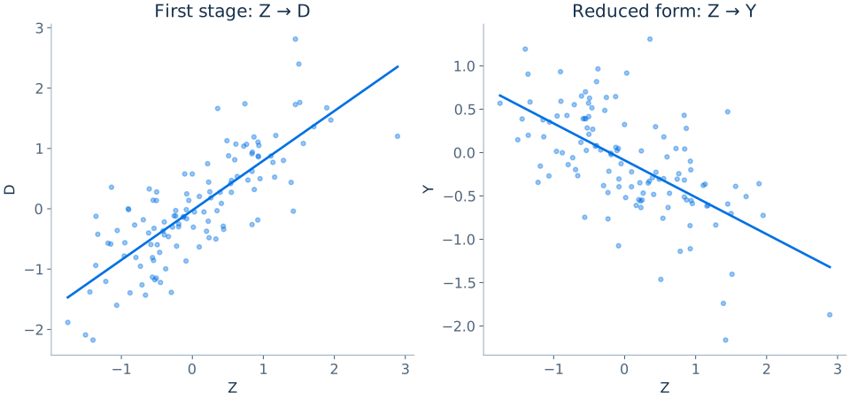
Identification and exclusion
Relevance can often be assessed using the data, but exclusion is rarely completely testable and requires institutional reasoning. Instruments may be weak despite statistically significant bivariate associations when the first stage is evaluated conditional on many controls. The direction and size of first-stage coefficients also deserve economic scrutiny. An instrument that shifts both demand and supply, for example, will not isolate one curve by merely being correlated with price.
There are three common identification categories: underidentified when insufficient independent instrument variation exists, just identified when the number of valid instrument restrictions matches endogenous parameters, and overidentified when there are more instruments than endogenous parameters. Overidentification can enable specification checks, but it does not make instruments valid by default.
Weak instruments and the first-stage diagnostic
Weak instruments create finite-sample bias, potentially severe nonnormality and unreliable conventional t and Wald inference. First-stage F-statistics or corresponding conditional robust diagnostics assess relevance, but a universal threshold is not valid in all settings. The familiar F>10 rule is an approximate historical screening heuristic for restricted specifications, not a theorem ensuring correct coverage with heteroskedasticity, clustering or multiple endogenous regressors.
Where weak identification is plausible, report appropriate weak-instrument-robust tests or confidence sets, such as Anderson–Rubin-type procedures under suitable assumptions, and consider whether the empirical design is informative at all. Adding many marginally relevant instruments can make finite-sample performance worse rather than better.
Overidentification tests
With more instrument moment restrictions than structural coefficients, the Hansen J test can assess whether the collection of restrictions is mutually compatible with the specified model and covariance assumptions. A rejection signals that at least one maintained moment condition is inconsistent with the others or with model specification. Nonrejection does not prove validity: invalid instruments could share the same violation, or the test may have low power.
For a single just-identified endogenous regressor and one excluded instrument there is no overidentifying restriction to test. The relevant empirical task is to defend exclusion with subject-matter knowledge and scrutinise the effect of alternative instrument candidates.
Heterogeneous treatment effects and LATE
When the effect of D varies across individuals, IV need not identify the population ATE. With a binary instrument and treatment, potential-treatment monotonicity and other standard assumptions, the Wald ratio identifies the local average treatment effect (LATE): the average effect among compliers, who take treatment if encouraged and do not take it otherwise. This is a population defined by the instrument's effect on behaviour, not a random subset of everyone.
A different instrument may identify a different complier population and thus a different local effect even when both IV estimates are internally valid. Interpreting IV as a universally applicable effect requires considering population heterogeneity and the economic meaning of compliance.
Applying IV in R
The formula in the next example denotes y as outcome, d as endogenous regressor, x1+x2 as included exogenous controls and z as excluded instrument. Robust inference uses a suitable covariance function. With a credible panel or clustered design, replace the covariance approach accordingly.
library(AER)
iv <- ivreg(y ~ d + x1 + x2 | z + x1 + x2, data = dat)
summary(iv, diagnostics = TRUE)
library(lmtest)
library(sandwich)
coeftest(iv, vcov. = vcovHC(iv, type = "HC1"))
# Explain and inspect the first stage:
first_stage <- lm(d ~ z + x1 + x2, data = dat)
summary(first_stage)The geometry of first-stage relevance
After partialling out the included controls W, the first stage asks whether residualised instruments predict residualised endogenous variation. With one instrument Z and one endogenous regressor D, relevance is Cov(Z̃,D̃)≠0 after both are residualised on W. A nonzero unconditional correlation is not enough if its entire source comes from shared dependence on included controls. A good IV report checks the conditional first stage and the economic mechanism through which the instrument shifts treatment.
In the presence of multiple instruments, a first-stage regression may fit strongly because of instruments individually correlated with D, but identification still requires appropriate rank conditions for all endogenous regressors. For multiple endogenous variables, relevance is a multivariate condition and cannot be reduced to a single bivariate correlation.
IV precision and research design
Even with a genuinely valid instrument, IV estimates can be less precise than OLS because they use only the component of treatment variation predicted by the instrument. This is the price paid for isolating plausibly exogenous variation. Reporting an imprecise but credible estimate can be more scientifically informative than reporting a very precise but confounded OLS association. Comparisons between OLS and IV must consider not only bias but also different weighted effects under treatment-effect heterogeneity.
A numerical two-stage example
Consider an instrument that raises the fitted participation rate from 0.20 to 0.50 and raises the fitted outcome mean from 100 to 112. The reduced form is 12, and the first-stage change is 0.30; the just-identified IV slope is 40 outcome units per induced participation. Now suppose the participation shift were only 0.03 while the estimated reduced form remained 12. The ratio becomes 400, illustrating the explosive sensitivity of the Wald estimator to a weak denominator. This arithmetic does not mean 400 is a plausible effect: the small first stage may make conventional uncertainty approximations unreliable.
How an Anderson–Rubin confidence set is constructed
Consider one endogenous regressor D and a proposed coefficient b. Under the null that b is the true structural effect, subtracting bD from Y leaves a combination of exogenous controls and the structural disturbance. Valid excluded instruments should then have zero coefficients in a regression of Y−bD on those instruments and all included exogenous controls. An Anderson–Rubin test assesses that joint restriction without dividing by an estimated first-stage coefficient.
Invert the test by retaining every b that is not rejected at the chosen significance level. The resulting confidence set can be wide, disconnected or unbounded when the data contain little identifying information. These shapes are meaningful and should not be truncated to create a reassuring finite interval. The classical F version requires its normal and spherical-error assumptions; robust variants use covariance estimators suited to heteroskedasticity or clustering and corresponding asymptotic justification. Protection against weak relevance does not protect against an invalid exclusion restriction. State both the maintained instrument assumptions and the inferential procedure.
14. Time Series, AR Models and Forecasting
Dependence over time, stationarity, lag selection and honest forecasting
The nature of time-series variation
A time series is an ordered sequence of observations indexed by time, such as quarterly GDP, monthly inflation or daily asset returns. Unlike independent cross-sectional observations, adjacent observations often contain overlapping information: output today depends on yesterday's output, price levels inherit past changes and financial volatility can persist across periods. Statistical inference and prediction must account for this temporal structure rather than mechanically using formulas derived for independent observations.
A useful transformation is the first difference ΔYt=Yt−Yt₋1. For a positive series, Δln(Yt)=ln(Yt)−ln(Yt₋1) approximates the growth rate between t−1 and t. If Y is an index or total price level, a difference may be meaningful in level units, whereas a log difference measures a proportional change. Transformations can remove some forms of trend but can also change the economic question and introduce their own serial-correlation pattern.
Autocovariance, autocorrelation and stationarity
For a weakly stationary process, the mean E[Yt]=μ is time-invariant, the variance is finite and constant, and the covariance between Yt and Yt₋k depends only on lag k, not on the date t. Denote this autocovariance γ(k)=Cov(Yt,Yt₋k). The autocorrelation is ρ(k)=γ(k)/γ(0). Positive first-order autocorrelation means that observations above the mean tend to be followed by further observations above the mean.
Nonstationary time series may have changing means, changing variance or persistent stochastic trends. A series displaying visual trend is not automatically a unit-root process; the distinction between deterministic and stochastic trends is important for transformations, hypothesis tests and forecast uncertainty.
The autoregressive model of order one
An AR(1) process has the form
where εt has conditional mean zero given information available at t−1. With |φ|<1 and white-noise innovations of variance σ2, the causal stationary solution has mean μ=c/(1−φ) and variance σ2/(1−φ2). These stationary moments apply when the process is initialised in its stationary distribution; an arbitrary initial value creates a transient. Conditional mean zero, which is stronger than simple lack of correlation with the past, justifies the conditional forecast below. For positive φ less than one, a shock gradually decays instead of disappearing immediately.
The k-step conditional forecast with known parameters is
Forecasts tend toward the long-run mean as k increases when |φ|<1. If φ approaches one, shocks decay very slowly and long-horizon uncertainty becomes substantial. At φ=1, the process is a random walk with drift: standard stationary AR formulas no longer apply.
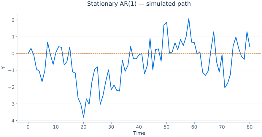
Autoregressions of higher order
An AR(p) model includes p lags of the dependent variable:
Higher lag orders allow richer persistence but add parameters and require a larger effective estimation sample. The relevant stability condition for AR(p) concerns the characteristic polynomial's roots, not merely whether each estimated coefficient individually has absolute value below one. The regression can be estimated by OLS under appropriate exogeneity of lagged predictors with respect to the current innovation and additional stationarity or regularity assumptions.
Model selection: AIC, BIC and validation
The lag order p can be chosen with information criteria that balance fit and model complexity. A common Gaussian-style form using a residual-variance estimate is
where kp counts fitted parameters and T is the effective sample size. Lower criterion values are preferred for the candidate set under the selected convention. BIC's penalty grows with ln T and more strongly favours parsimonious models as samples expand. For valid comparisons, lag candidates should be evaluated on comparable estimation samples and criteria must use compatible normalisations.
Time-series cross-validation should preserve chronological order. One strategy is rolling-origin evaluation: estimate using data available up to date t, forecast t+1, move forward and repeat. This provides a practical estimate of performance under genuine future prediction. Random-fold cross-validation can leak future information if the folds break temporal structure.
MSFE, forecast uncertainty and benchmarks
For h-step forecasts Ŷt₊h|t, forecast errors are et₊h=Yt₊h−Ŷt₊h|t. Mean squared forecast error is MSFE=(1/m)Σe2 over genuine evaluation dates. A good benchmark may be a historical average, random walk or simple AR model. Sophisticated models should be judged against credible simpler alternatives using data not employed in estimation.
Forecast intervals require accounting for innovation uncertainty, parameter uncertainty and possible model instability. In a stationary AR(1) with known φ and innovations having constant conditional variance σ2 and zero conditional mean, the k-step innovation forecast-error variance is
Longer horizons ordinarily accumulate uncertainty. If the model parameters are estimated, additional uncertainty must be considered when the sampling scale makes it material.
Unit roots and spurious regression
A random walk Yt=Yt₋1+εt has a unit root and is not weakly stationary. Regressing one unrelated trending series on another can produce apparently impressive t-statistics and R2 values even though the underlying innovations are independent—a spurious regression. Unit-root tests have nonstandard reference distributions and should not be interpreted like ordinary regression t-tests. Differencing can recover a stationary process in some cases, but differencing a genuinely stationary trend-adjusted relationship can discard valuable information.
When two nonstationary series share a stable long-run equilibrium relationship, they may be cointegrated. An error-correction model can represent both short-run changes and adjustment toward the long-run equilibrium. This is a substantial extension; simply finding a statistically significant regression between two price levels is insufficient evidence of cointegration.
Practical forecasting in R
The following illustrates AR fitting, time-aware training and basic diagnostic thinking. Real research should check seasonal effects, residual autocorrelation, structural breaks and forecast stability.
# Assume y is a numeric time-series vector ordered chronologically.
y_train <- head(y, length(y) - 12)
y_test  <- tail(y, 12)
fit_ar <- arima(y_train, order = c(1, 0, 0), include.mean = TRUE)
fc <- predict(fit_ar, n.ahead = 12)
rmse <- sqrt(mean((y_test - fc$pred)^2))
print(rmse)
acf(residuals(fit_ar))Dynamic effects and distributed-lag models
An economy may not respond fully to a policy in the same period it occurs. A distributed-lag model describes the outcome as a function of current and lagged explanatory variables, such as
Here δ0 is the contemporaneous response holding other explanatory terms fixed, while δ1 and δ2 capture further responses at later horizons under the model's timing interpretation. If a permanent one-unit increase in X persists from period t onward, the cumulative response after all included lags have taken effect is δ0+δ1+δ2. The standard error of this sum must include covariances among lag-coefficient estimates.
For causal interpretation, the input sequence X must be exogenous in a sufficiently strong sense relative to unobserved shocks. Lagging a regressor does not automatically eliminate endogeneity: agents may anticipate shocks, policies may respond to past disturbances and persistent unobserved conditions may correlate with present values of X.
Forecast comparison and structural breaks
A structural break occurs when the mean, variance or predictive coefficients change. An AR model fitted entirely before a major reform can forecast poorly afterward even with low historical residual error. Rolling evaluations and stability tests are therefore central to forecast reliability. A model can have excellent one-step forecasts but deteriorate at longer horizons because small dynamic errors accumulate. Always report the horizon, training window and forecast benchmark; claiming a forecasting model is “accurate” without these details is incomplete.
Testing for a unit root: the null hypothesis matters
The augmented Dickey–Fuller regression explains the first difference using a lagged level, optional deterministic terms and lags of the first difference. In the equation below, the unit-root null is γ=0. The stationary alternative has a negative adjustment coefficient in the appropriate stable specification. The constant, trend and lag order influence the reference distribution and the interpretation; an ordinary Student t critical value is inappropriate.
Failure to reject a unit root does not prove its presence, especially in short or highly persistent series. Conversely, the KPSS test starts from a stationarity null, so its p-value answers a different question. Conflicting results should prompt examination of structural breaks, deterministic trends and finite-sample power, rather than a majority vote between tests. Too much differencing can introduce unnecessary serial correlation and remove economically meaningful level relationships. In R, tseries::adf.test includes a constant and linear trend by default; this choice should be understood rather than mistaken for a neutral test of every possible deterministic specification.
| Test | Null hypothesis | Meaning of rejection |
|---|---|---|
| ADF | Unit root under the specified deterministic terms | Evidence against that unit-root model |
| KPSS | Level or trend stationarity, depending on specification | Evidence against that stationarity model |
15. Panel Data, First Differences and Fixed Effects
Using within-unit variation to control for time-invariant heterogeneity
Why panels change the identification problem
Cross-sectional regressions compare different individuals, firms or regions. If units have enduring but unobserved characteristics, such as managerial skill, institutional quality or longstanding preferences, these factors may confound cross-sectional associations. Panel data repeatedly observe the same units and make it possible to remove fixed unobserved characteristics through within-unit comparisons. This advantage comes with new assumptions about time-varying confounding and dependence within units.
The canonical additive fixed-effects model is
Here αi is a time-invariant unit effect, λt is a time effect shared across units, and uit is the remaining time-varying disturbance. The coefficient β is identified by within-unit changes in X after adjusting for common time shocks under the relevant exogeneity assumptions. A variable that never changes within an individual cannot have its own slope separately identified in a model with unrestricted unit fixed effects.
First differencing with two periods
For two periods, start with Yi1=αi+βXi1+ui1 and Yi2=αi+βXi2+ui2. Subtract the first from the second:
The unobserved αi disappears exactly. OLS on differences consistently estimates β when changes in X are appropriately exogenous with respect to changes in the disturbance. A constant unobserved individual characteristic need not be uncorrelated with X in levels, which is the key attraction of the method.
However, first differencing does not remove unobserved time-varying factors. If a firm changes investment because an unrecorded demand shock raises its expected sales, that shock may affect both ΔX and ΔY. Measurement error can also become more important after differencing because signal in a persistent variable is reduced while measurement noise remains.
Fixed-effects (within) estimation
For more than two periods, take each individual's time average. The model Yit=αi+βXit+uit implies Ȳi=αi+βX̄i+ūi. Subtract the average equation from each period:
OLS on these demeaned data estimates the within-unit slope. An equivalent least-squares dummy variable estimator includes an intercept for each unit except an omitted reference, when feasible. Both estimators remove additive time-invariant αi and yield the same slope under corresponding specifications.
The standard assumption for the static FE model is often strict exogeneity: E[uit|Xi1,…,Xit,…,XiT,αi]=0 for every t. This requires every disturbance uit to have mean zero conditional on the entire regressor history, including future X values. In particular, it rules out feedback in which a shock today changes next period’s regressor; it is stronger than the sequential exogeneity sometimes used in dynamic time-series models. A lagged dependent variable with fixed effects creates additional complications in short panels.
Unit and time fixed effects
Adding λt adjusts for common shocks or trends affecting all units. A two-way fixed-effects regression with unit and time dummies is
In the absence of other controls, β compares changes within units relative to the corresponding changes in other units that identify the regression. Two-way FE can be a useful descriptive control strategy, but under staggered policy adoption and heterogeneous dynamic treatment effects, its coefficient need not equal a transparent, convex weighted average of treatment effects. Modern difference-in-differences methods may be preferable for such designs.
Difference-in-differences
With treated and control units observed before and after a policy, the basic DID estimator is
The critical parallel-trends assumption says that, without treatment, treated and control units would have experienced the same expected change in the outcome over the comparison period. This is about unobserved counterfactual changes; pre-policy trends can provide useful evidence but cannot logically prove the counterfactual assumption for the post-policy period.
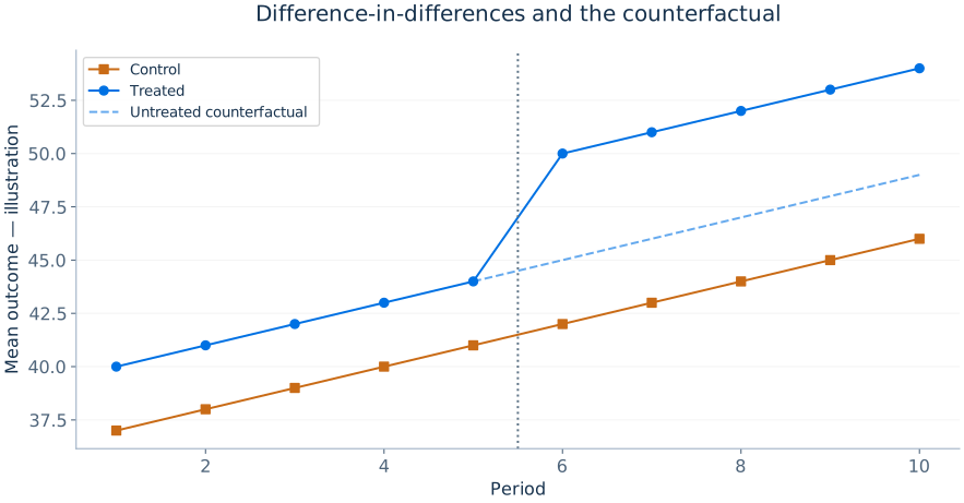
Random effects and correlated random effects
A conventional random-effects model treats the individual effect as uncorrelated with explanatory variables, allowing a weighted combination of within- and between-unit information. When this exogeneity holds, RE can be more efficient than FE. When αi correlates with X, standard RE can be inconsistent while FE can remain consistent under its own assumptions. A correlated random-effects or Mundlak specification includes unit-level means of time-varying regressors to model the dependence between αi and X. Such formulations can connect FE and RE and provide meaningful additional parameters in certain settings.
Model choice is not settled solely by a mechanical Hausman test. The assumptions, the effects of interest, whether time-invariant regressors matter and the clustering structure all deserve attention.
Serial correlation and clustered inference
Observations from the same unit over time are rarely independent. A FE regression usually requires standard errors clustered by unit, under a large-cluster asymptotic framework and assumptions of independence across clusters. If shocks are also correlated across units at a date, the dependence may require additional adjustment or a different inferential strategy. Unbalanced panels are often estimable, but attrition related to unobserved potential outcomes can affect interpretation.
library(fixest)
fe <- feols(y ~ x1 + x2 | firm_id + year, data = dat,
            vcov = ~ firm_id)
summary(fe)
# A DID specification when policy adopts at a common date:
did <- feols(y ~ treated:post | firm_id + year,
             data = dat, vcov = ~ firm_id)
summary(did)A worked fixed-effects transformation
Suppose two regions are observed in three years, and the researcher wants to estimate the relationship between policing and crime. The first region has a permanently higher baseline crime level because of unmeasured historical conditions; the second region has permanently lower baseline crime. A pooled regression may confuse these fixed differences with policing if police resources are also systematically higher in the first region. Region fixed effects subtract each region's own mean from outcomes and regressors, leaving only deviations within that region over time.
This procedure does not make an increase in policing exogenous. If a region hires extra police in anticipation of a crime wave, the within-region policing change may still correlate with the unobserved impending shock. A stronger source of identification might be a funding formula, a predetermined staffing shock or another externally motivated policy change. Fixed effects remove fixed confounding, not policy responsiveness.
Clustering and effective information in panels
Repeated observations on the same region or firm share unobserved influences, so a regression with thousands of firm-year rows but only 20 firms may have less independent information than the raw row count suggests. The level of clustering should reflect the assignment and shock mechanisms. If a reform is assigned at the region level, clustering at an individual worker level is usually inadequate because treatment variation and shared shocks occur at the region level. If both region and year shocks exhibit complex dependence, more sophisticated inference may be needed.
Treatment timing, cohort effects and event-time comparisons
Let Gi denote the first period in which unit i is treated. The group-time effect ATT(g,t) compares the average outcome at date t for the cohort first treated in g with its counterfactual outcome if it had remained untreated. This target allows the effect to differ across cohorts and with exposure duration. Identification needs an appropriate parallel-trends assumption, no anticipation over the specified window, suitable overlap and an untreated comparison group.
For example, a cohort treated in 2023 can be compared in 2024 with units still untreated in 2024, if those units provide a credible counterfactual. Units treated in 2022 are already exposed; using them as controls can subtract their evolving treatment effects. Cohort-time estimators make this comparison explicit before aggregating. Event time e=t−g measures duration since adoption, whereas calendar time t locates common shocks. Aggregation should disclose cohort weights and which cohorts remain observed at each horizon. Non-rejection of pre-treatment differences supports a limited diagnostic; it does not establish parallel counterfactual trends after treatment.
16. Shrinkage, Big Data and Regularised Prediction
Ridge, Lasso, cross-validation and principal components
Prediction with many potential regressors
The number of available predictors may become large relative to the number of observations. Advertising campaigns, consumer purchases and macroeconomic forecasts can be described by hundreds of covariates and lags. An unrestricted OLS regression can fit training data extremely closely yet produce poor out-of-sample performance because its coefficients respond to sampling noise. Regularisation deliberately introduces bias to reduce variance and potentially improve prediction.
A predictive model and a causal model are judged by different criteria. A useful predictor need not cause an outcome: it may simply be an early or correlated signal. For example, web searches may help forecast sales without being a manipulable determinant of consumption. A well-designed causal estimate instead requires a defensible counterfactual comparison, often with a carefully structured adjustment set.
Bias–variance trade-off
For a new observation with covariates X0, a predictive estimate ŷ(X0) has mean squared error composed of squared bias, variance and irreducible outcome noise under suitable conditioning. Increasing model flexibility can reduce approximation bias but increase estimation variance. A very complicated model may capture idiosyncratic patterns in the training sample that do not recur in fresh observations. Shrinkage aims to control that trade-off.
Ridge regression
Ridge minimises the OLS loss plus a squared-coefficient penalty:
The intercept is usually left unpenalised and the explanatory variables are standardised before fitting. The tuning parameter λ≥0 controls the amount of shrinkage: λ=0 recovers OLS under full rank; larger λ moves slope coefficients toward zero. For centred X and Y, the matrix form is β̂ʳⁱᵈᵍᵉ=(X′X+λI)-1X′y. Ridge stabilises near-collinear designs but typically does not set individual coefficients exactly to zero.
Lasso and sparse models
Lasso replaces the squared penalty by the absolute-value penalty Σ|βj|, enabling variable selection through exact zero coefficients. When a relatively small number of predictors carry most of the useful signal, Lasso can give a compact forecasting model. It is not automatically superior to ridge: highly correlated blocks of predictive variables can lead to unstable selection, while ridge may distribute coefficient weight more smoothly. Elastic net combines L1 and L2 penalties and can be valuable when many correlated predictors are present.
The tuning parameter is not estimated from ordinary OLS t-statistics. It is commonly chosen to minimise cross-validated prediction loss. Choosing both the variable transformations and the penalty by repeatedly checking the same test sample leads to evaluation leakage. A genuine holdout dataset should remain unused until final evaluation.
K-fold cross-validation
Divide the training sample into K folds. For each candidate λ, fit the model on K−1 folds and predict observations in the held-out fold. Average the holdout losses across folds and choose a penalty with satisfactory cross-validated performance. Finally refit on the entire training sample and evaluate once on an untouched test set. Nested validation or a separate validation stage may be helpful when many hyperparameters and model families are compared.
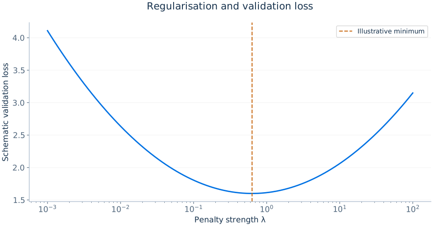
Principal components
Principal component analysis transforms a vector of correlated regressors into orthogonal linear combinations ranked by the amount of predictor variance they explain. If the standardised data matrix is X, the principal-component directions solve an eigenvector problem for X′X or the corresponding covariance matrix. A prediction model can regress Y on a limited number of leading components. This may reduce dimensionality, but the components explaining most variation in X do not necessarily explain most variation in Y, so the number of components should be selected for the predictive task.
Time-series prediction with many predictors
Macroeconomic forecasting may employ many correlated series such as employment, confidence, production, prices and financial indicators. Dynamic factor models assume that much of their joint variation reflects a smaller number of latent factors. Factor-based forecasts can reduce estimation complexity while exploiting a wider information set, but data revisions, changes in relationships and future-data leakage complicate evaluation.
Simple implementation in R
The following schematic example assumes complete data and numeric predictors with identical names and order in train and test. glmnet standardises predictors internally by default. With factors, build the test matrix using the training terms, factor levels and contrasts, then verify identical columns; two separate model.matrix calls alone do not guarantee compatible encoding. Use the same prespecified folds to compare ridge with Lasso, and keep test outcomes out of every tuning decision.
library(glmnet)
X <- model.matrix(y ~ . - 1, data = train)
y <- train$y
set.seed(2026)
fold_id <- sample(rep(seq_len(10), length.out = nrow(X)))
ridge <- cv.glmnet(X, y, alpha = 0, foldid = fold_id)
lasso <- cv.glmnet(X, y, alpha = 1, foldid = fold_id)
coef(lasso, s = "lambda.min")
newX <- model.matrix(y ~ . - 1, data = test)
stopifnot(identical(colnames(X), colnames(newX)))
pred <- as.numeric(predict(lasso, newx = newX, s = "lambda.min"))
sqrt(mean((test$y - pred)^2))Ridge shrinkage and singular values
Let the centred design matrix have singular value decomposition X=UΣV′. Ordinary least squares in its principal directions multiplies components of the outcome by the reciprocal of singular values. When a singular value is very small, tiny fluctuations in the outcome can create large coefficient changes. Ridge modifies the contribution by replacing the unstable inverse weighting with factors σj/(σj2+λ), damping directions with weak predictor variation. This explains why ridge often performs well with collinear economic indicators.
The penalty λ should be selected on training data, and model assessment should use genuinely new observations. Inference on individual ridge or Lasso coefficients is not obtained by reading conventional OLS t-statistics off a selected model; the regularisation bias and selection stage require specialised methods.
Choosing prediction tools for a specific task
Use simple OLS when predictors are few, relationships are approximately linear and extrapolation or interpretation is important. Consider ridge when many predictors are correlated and forecasting dominates variable selection. Consider Lasso when a sparse predictive representation is plausible and a compact specification is valuable. Principal components may help when many indicators share a few latent factors; dynamic factor models extend this intuition to time-dependent macroeconomic panels.
17. Experimental and Quasi-Experimental Reasoning
Counterfactual identification, LATE, matching and regression discontinuity
A design-based way to think
The central challenge in applied econometrics is not the calculation of a regression coefficient but the construction of a credible comparison. In an ideal randomised controlled trial, assignment to treatment is independent of potential outcomes. In observational studies, researchers seek circumstances in which treatment changes for reasons plausibly unrelated to the unobserved outcome determinants. Identifying such variation may depend on a regulation, an institutional threshold, a natural event or a policy timetable; each source has its own assumptions and threats.
The relevant objects should be named precisely: a sample average treatment effect (SATE) refers to the realised study sample; a population ATE averages across the population; ATT refers to the treated; and IV may identify LATE for compliers. These parameters differ when effects vary with people, treatment intensity or baseline circumstances. Researchers should not treat every estimate as a universal treatment effect.
Randomised experiments and intention to treat
With random assignment Z to a programme, the intention-to-treat effect is the difference in mean outcomes by assignment:
It measures the effect of offering or assigning treatment, regardless of actual take-up, assuming the experiment's integrity and correct outcome measurement. If assignment changes participation D but not everyone complies, the Wald ratio ITT of Y divided by ITT of D can identify LATE under the standard additional assumptions: random assignment, exclusion, relevance and monotonicity. ITT and the effect of receiving treatment answer different questions and should be reported accordingly.
Experiments can be distorted by selective attrition, treatment contamination, spillovers and departures from the assigned protocol. Randomisation addresses baseline confounding in expectation; it does not make badly measured post-treatment outcomes reliable or guarantee that results transport to another country.
Matching, regression adjustment and overlap
If treatment is conditionally independent of potential outcomes given observed pretreatment X and overlap holds, treated and untreated units can be compared within sufficiently similar control strata. Matching methods construct comparisons based on observed characteristics or a propensity score e(X)=P(D=1|X). Regression adjustment models expected outcomes given controls and treatment status. Inverse-probability weighting reweights observations according to treatment propensity.
Matching and regression do not produce causal validity by themselves. Both depend on the claim that the observed controls eliminate selection bias and must be sensitive to lack of overlap, model misspecification and poor measurement. Weighting can become unstable when propensity scores approach zero or one. Before fitting a model, inspect which combinations of covariates appear in both groups and whether the implied counterfactual comparisons are credible.
Regression discontinuity designs
A regression discontinuity (RD) design exploits an assignment rule that changes at a known threshold c of a running variable R. For a sharp RD, treatment changes deterministically at c, so the causal effect at the cutoff is identified as the discontinuity in the conditional expectation:
The crucial assumption is continuity of potential-outcome expectations in the running variable at the threshold in the absence of treatment. Units immediately on either side should be comparable except for treatment. Estimation usually uses local polynomial methods in a neighbourhood of c, bandwidth selection and inference procedures suited to the local design. A global high-order polynomial fit is generally a poor substitute for careful local analysis.
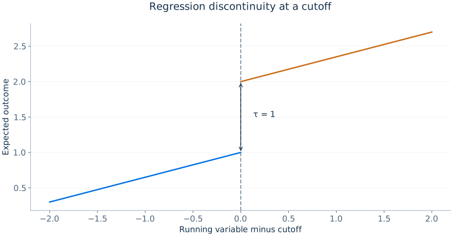
In a fuzzy RD, treatment probability jumps at the cutoff without switching perfectly from zero to one. The jump in outcomes is divided by the corresponding jump in treatment probability, making fuzzy RD a local instrumental-variable design. Manipulation or strategic sorting around the threshold, other concurrent policy cutoffs and discontinuous baseline covariates threaten validity.
Difference-in-differences revisited
A policy adopted in one region but not another may create a natural experiment if untreated potential outcomes follow comparable trends. DID subtracts the comparison region's change from the treated region's change, removing fixed group differences and common time shocks in the basic setup. An event-study model can estimate relative effects before and after treatment, but its interpretation requires appropriate treatment-effect heterogeneity handling and no differential anticipatory responses.
Where treatment adoption varies across periods and groups, ordinary two-way FE can yield misleading weighted averages under heterogeneous effects. Estimators designed to compare newly treated units with appropriate untreated or not-yet-treated controls may provide more transparent targets.
Design diagnostics and honest interpretation
Each identification strategy has a distinct place for empirical diagnostics: balance and attrition in experiments, overlap and covariate balance in matching, pre-policy trend evidence in DID, density and covariate continuity at the RD threshold, and first-stage strength plus exclusion arguments for IV. None of these diagnostics proves every causal assumption; their value is in ruling out particular plausible failures and making the study's limitations transparent.
A useful research report connects: research question → estimand → identifying comparison → estimation method → standard error → economic interpretation → limitations. Sophisticated estimators cannot substitute for this sequence.
18. Applied Econometrics with R
A reproducible workflow from raw data to defensible regression tables
Reproducibility and the analysis pipeline
Applied econometrics is a computational discipline. Reliable results require more than a single successful regression command: data origins, transformations, missing-value decisions, sample construction, model formulas and the chosen standard-error estimator must be documented. A reproducible script should start from the same raw input files, perform all cleaning transformations explicitly and recreate estimates, diagnostic plots and final tables without manual edits.
R is an open-source programming environment for data analysis. The familiar workflow uses a script editor such as RStudio, CSV or other data imports, objects holding data frames and models, and packages for inference or visualisation. The basic modelling command lm estimates OLS. The formula y ~ x1 + x2 includes an intercept by default; y ~ x1 + x2 - 1 removes it. Syntax should never be mistaken for identification: the model formula encodes variables, not whether their coefficients have causal interpretations.
A minimal reproducible project
The following script uses an explicitly synthetic sample. It is intended to demonstrate software behaviour, not to emulate the coefficients of a particular empirical textbook dataset. Because the random seed is fixed, running the code on a compatible installation should reproduce the same generated observations.
set.seed(2026)
n <- 500
education <- round(pmin(20, pmax(8, rnorm(n, 13, 2))))
experience <- runif(n, 0, 30)
ability <- rnorm(n)
logwage <- 1.6 + 0.07 * education + 0.02 * experience +
           0.12 * ability + rnorm(n, sd = 0.30)
dat <- data.frame(education, experience, ability, logwage)
summary(dat)
plot(dat$education, dat$logwage, pch = 19, cex = .5,
     xlab = "Years of education", ylab = "Log wages")
In this data-generating process, the structural conditional education coefficient is 0.07 when ability and experience are included. Altering the simulation so ability also influences education would create omitted-variable bias in an education-only regression. Simulated examples are useful because the researcher knows the truth and can assess estimation behaviour rather than guessing it from the fitted output.
Simple versus multiple regression
m1 <- lm(logwage ~ education, data = dat)
m2 <- lm(logwage ~ education + experience + ability, data = dat)
summary(m1)
summary(m2)
confint(m2)
Compare the education coefficients, the estimated residual scale and the confidence intervals. The discrepancy between simple and multiple slopes reveals how adjustment changes conditional comparisons; it is not automatically a proof of the direction or magnitude of omitted confounding in an unrelated observational dataset. Next modify the simulation so that education depends on ability and evaluate how the estimates change across repeated samples.
Transformations and interactions
m3 <- lm(logwage ~ education + experience + I(experience^2), data = dat)
m4 <- lm(logwage ~ education * ability + experience, data = dat)
summary(m3)
summary(m4)
# Marginal effect of experience at a selected experience level:
b <- coef(m3)
me_exp_10 <- b["experience"] + 2 * b["I(experience^2)"] * 10
print(me_exp_10)
R's I() operator treats a mathematical expression as a single transformed predictor, while x1 * x2 expands to the main effects and interaction (x1 + x2 + x1:x2). A marginal-effect estimate is a function of several coefficients; calculate its uncertainty with the model covariance matrix rather than treating the components as independent.
Robust and clustered inference
library(lmtest)
library(sandwich)
coeftest(m2, vcov. = vcovHC(m2, type = "HC3"))
# For genuine clustered data with independent clusters:
# coeftest(m2, vcov. = vcovCL(m2, cluster = dat$cluster_id))
The HC3 estimate changes the estimated standard errors and test statistics, not the OLS coefficients. Cluster-based methods require an actual cluster identifier and a sampling structure that supports cluster-asymptotic inference. Inventing a cluster ID simply to obtain different standard errors would have no statistical justification.
General linear restrictions
The car package provides convenient Wald tests under the supplied covariance matrix. When testing several restrictions jointly with heteroskedasticity, it is important to request a robust covariance matrix rather than silently relying on the classical regression ANOVA table.
library(car)
linearHypothesis(m2, c("education = 0", "experience = 0"),
                 vcov. = vcovHC(m2, type = "HC3"))
Instrumental variables
For a real IV analysis, articulate why the excluded instrument affects the endogenous regressor and why it cannot affect the outcome through other channels. R formula notation in ivreg() separates the structural regression from the instrument set with |. The instrument set contains the excluded instruments and all included exogenous controls.
library(AER)
# Illustrative schema: z is an externally justified instrument for d
iv_fit <- ivreg(y ~ d + income + age | z + income + age,
                data = empirical_data)
summary(iv_fit, diagnostics = TRUE)
coeftest(iv_fit, vcov. = vcovHC(iv_fit, type = "HC1"))
This second template is intentionally not executable until the analyst supplies a real data frame with justified variable definitions. Running a regression without a credible instrument does not create a meaningful causal estimate.
Panel models
The fixest package provides concise estimation of unit and time fixed effects. A vertical bar inside feols separates regressors from fixed-effect dimensions. Clustering by unit allows flexible residual dependence within each unit, under the corresponding assumptions.
library(fixest)
model_fe <- feols(outcome ~ policy + control1 | region + year,
                  vcov = ~ region, data = panel_dat)
etable(model_fe)
If treatment changes by region and year, interpret the coefficient in light of the assignment mechanism and whether an ordinary FE parameter represents the desired causal estimand. When the research question is DID with staggered treatment, dedicated estimators may be needed rather than simply adding more fixed effects.
Model diagnostics and plots
par(mfrow = c(2, 2))
plot(m2)
par(mfrow = c(1, 1))
# Save a reproducible data summary:
capture.output(summary(dat), file = "descriptive_summary.txt")
The base R diagnostic suite includes residual-versus-fitted, Q–Q, scale-location and leverage-related plots. A residual–fitted plot may reveal nonlinearities and heteroskedasticity. Normal Q–Q departures deserve attention for exact small-sample inference but do not automatically invalidate a large-sample robust regression. Influential observations need substantive inspection instead of automatic deletion.
Reporting numerical results without overclaiming
A good empirical table names the dependent variable, the estimation method, standard errors (including their clustering level), observation count, fixed effects, important controls, and estimation sample. Accompany each major coefficient with a correctly unit-labelled interpretation and a discussion of causal identification. For interaction and log models, convert coefficients into marginal effects on meaningful scales. Specify the population and time period, and state where data or methods restrict generalisability.
| Step | Essential action | Diagnostic question |
|---|---|---|
| Data | Inspect, clean, transform | Are units and missing values understood? |
| Design | Define estimand and controls | Is variation plausibly exogenous? |
| Estimate | Choose OLS, IV, FE or other | Does method target the stated parameter? |
| Infer | Choose robust or clustered covariance | Are observations statistically independent? |
| Validate | Check specification and sensitivity | Could assumptions fail? |
| Communicate | Report coefficient, uncertainty and scope | What can the result genuinely establish? |
A clean estimation sample and a reproducible prediction pipeline
Before comparing specifications, define the observation key and verify that it is unique. A firm-year panel should have one intended record per firm-year; a many-to-many merge can silently multiply observations and distort both coefficients and standard errors. Record the units, date range, outcome definition, missingness by variable and every sample restriction. A coefficient can change after adding a control because the model now uses a different sample, so compare nested specifications on a common sample when isolating the role of adjustment.
For prediction, divide data into training, validation and test portions according to the deployment setting. Fit imputation rules, scaling, feature selection and learned transformations using training data only, then apply the fitted rules to held-out data. Preserve training factor levels, contrasts, column names and column order. Repeated units should remain together when the goal is prediction for unseen units, and future dates must stay out of earlier forecasting folds. Save the random seed, package versions, model formula, preprocessing objects and final sample count. These records make a result reproducible; they do not replace a defensible identification argument.
| Check | Why it matters |
|---|---|
| Unique observation keys | Prevents accidental multiplication of rows after joins |
| Common estimation sample | Separates changes in controls from changes in observations |
| Training-only preprocessing | Prevents information from held-out outcomes or covariates leaking into fit |
| Matching model-matrix columns | Preserves the meaning and order of trained coefficients |
| Saved seed and package versions | Makes stochastic and software-dependent steps traceable |
19. Mathematical Toolkit and Worked Problems
Essential derivations, numerical exercises and fully explained solutions
Summation and matrix identities
In econometrics, Σi denotes summation over observed units. A vector is an ordered collection of values, a matrix is a rectangular array and the transpose X′ interchanges its rows and columns. The inverse (X′X)-1 exists only when X′X has full rank. In OLS, fitted values are orthogonal projections, so Px=Px′ and Px2=Px; this idempotence explains many algebraic least-squares identities.
For ordinary scalar variables with finite moments, covariance is Cov(X,Y)=E[XY]−E[X]E[Y]. The population simple-regression slope minimising E[(Y−a−bX)2] is Cov(X,Y)/Var(X) whenever Var(X)>0. The numerator determines direction and the denominator rescales variation in X. Conditional expectation E[Y|X] minimises E[(Y−g(X))2] across all measurable functions g with appropriate finite second moments; linear regression restricts g to a linear class.
Deriving the simple-regression OLS formula
Start with S(a,b)=Σ(Yi−a−bXi)2. The first-order condition in a is −2Σ(Yi−a−bXi)=0. Dividing by n gives Ȳ−a−bX̄=0, so a=Ȳ−bX̄. The first-order condition in b is −2ΣXi(Yi−a−bXi)=0. Replace a by the previous expression, expand centred variables and rearrange to obtain b=Σ(Xi−X̄)(Yi−Ȳ)/Σ(Xi−X̄)2. The second derivative in the slope is positive if the X values are not all equal, ensuring a unique minimiser.
Deriving the variance of a two-variable linear combination
For constants a and b and random variables X and Z,
Expand the squared deviation from the mean and use linearity of expectation. This identity appears repeatedly in econometrics: the standard error of a linear combination of regression coefficients, the predicted effect of an interaction and the variance of a portfolio all depend on covariance terms. Assuming coefficients are uncorrelated without checking the variance-covariance matrix is a common mistake.
Deriving the OLS asymptotic variance
From β̂−β=[(1/n)ΣXiXi′]-1(1/n)ΣXiui, multiply by √n. Under regularity conditions, the matrix of regressors converges to Q and the score average satisfies a multivariate CLT, (1/√n)ΣXiui→ᵈN(0,Ω). Slutsky's theorem gives √n(β̂−β)→ᵈN(0,Q-1ΩQ-1). This result makes clear both why standard errors typically shrink at the rate 1/√n and why heteroskedasticity affects Ω. It also clarifies that an asymptotic variance formula is not a claim of finite-sample unbiasedness.
Worked exercise: a fitted regression line
Problem. Observe X=(0,1,2,3) and Y=(1,2,2,5). Calculate β̂1 and β̂0, residuals and R2.
Solution. X̄=1.5 and Ȳ=2.5. The centred cross-product sum is (−1.5)(−1.5)+(−0.5)(−0.5)+(0.5)(−0.5)+(1.5)(2.5)=6.0. The squared-X deviations sum to 5, so β̂1=1.2 and β̂0=0.7. Fitted values are (0.7,1.9,3.1,4.3), and residuals (0.3,0.1,−1.1,0.7). RSS=0.09+0.01+1.21+0.49=1.8. TSS=2.25+0.25+0.25+6.25=9, giving R2=1−1.8/9=0.80. The residuals add to zero as expected for OLS with an intercept.
Worked exercise: a joint hypothesis
Problem. An unrestricted model has RSSu=120 with n=100 observations and k=4 nonconstant regressors. A restricted model imposes q=2 restrictions and has RSSr=144. Compute the conventional partial F statistic.
Solution. The unrestricted residual degrees of freedom are 100−4−1=95. The fit penalty per restriction is (144−120)/2=12, while the unrestricted residual mean square is 120/95=1.2632. Therefore F=12/1.2632=9.50, to compare with the relevant F(2,95) critical value under the classical assumptions. If heteroskedasticity is present, this RSS-based reference distribution may be inappropriate; a robust Wald test is required.
Worked exercise: interpreting a log-level specification
Problem. A fitted regression gives ln(wage)=1.8+0.06education. Estimate the exact fitted wage ratio for an additional three years of schooling.
Solution. The change in fitted ln wage is 3×0.06=0.18. The ratio of exponentiated fitted log wages is exp(0.18)≈1.1972, a 19.72% difference; the first-order approximation is 18%. This is a ratio of conditional geometric means when the log conditional mean is correctly specified. It also represents the ratio of conditional arithmetic means only when the retransformation factor E[exp(u)|education] is unchanged across the comparison. A causal interpretation additionally requires exogeneity, which the fitted equation does not establish.
Worked exercise: omitted-variable bias
Problem. The true model is Y=β0+2X+3Z+u, and Cov(X,Z)/Var(X)=−0.4. Find the population coefficient from a simple regression omitting Z.
Solution. β̃1=2+3(−0.4)=0.8. The observed slope understates the direct X effect because the omitted factor raises Y while tending to be lower among observations with higher X. The sign analysis should precede arithmetic: a positive omitted effect multiplied by negative X–Z association produces negative bias.
Worked exercise: treatment selection
Problem. Treated and untreated average outcomes are 18 and 15. The treated population would have averaged 16 without treatment. Compute ATT and selection bias.
Solution. ATT=18−16=2. Selection bias=16−15=1. The observed contrast of 3 equals 2+1. Treating the raw difference as causal exaggerates the ATT by 50% in this example.
Worked exercise: an IV ratio
Problem. A randomly assigned programme offer increases training participation by 0.20 and average annual earnings by €360. Under relevance, exclusion, monotonicity and random assignment, interpret the Wald estimator.
Solution. The IV estimate is 360/0.20=€1,800. Under the assumptions and appropriate treatment definition, it identifies an average effect of actual training for compliers whose treatment status is changed by the offer. It does not directly estimate the effect for always-takers, never-takers or the whole eligible population unless stronger homogeneity assumptions hold.
Worked exercise: panel first differences
Problem. Three firms have (X1,Y1)=(1,5),(2,9),(4,12) and (X2,Y2)=(2,7),(4,12),(5,13). Compute the observed changes, and explain why regressing ΔY on ΔX can be useful.
Solution. ΔX=(1,2,1) and ΔY=(2,3,1). If the model has an additive time-invariant firm effect, that unobserved effect disappears when outcomes and regressors are differenced. A regression on changes therefore uses within-firm rather than between-firm information, but a causal interpretation still requires ΔX to be sufficiently exogenous with respect to Δu.
Worked exercise: the omitted covariance term
Problem. An interaction estimate has β̂1=2, β̂3=0.5, Var(β̂1)=0.16, Var(β̂3)=0.01 and Cov(β̂1,β̂3)=−0.02. Find the estimated treatment effect and standard error at X=3.
Solution. The effect is 2+3×0.5=3.5. Its variance is 0.16+9×0.01+2×3×(−0.02)=0.13, so SE≈0.3606. Ignoring the negative covariance would instead yield √0.25=0.5 and materially overstate the uncertainty for this particular contrast.
Further guided exercises
Exercise A. Derive why the OLS sample residual mean is zero when an intercept is included. Answer. The first-order condition for the intercept is Σûi=0; divide by n. Exercise B. Show that multicollinearity does not itself bias OLS under zero conditional mean. Answer. Conditional expectation E[β̂−β|X]=(X′X)-1X′E[u|X]=0 whenever the matrix is invertible; collinearity affects that inverse and therefore precision.
Exercise C. Explain why a positive first-stage effect and a negative reduced form imply a negative just-identified IV slope. Answer. Their ratio is negative; the exclusion argument is still needed for causal interpretation. Exercise D. Explain why predictive cross-validation does not establish IV exclusion. Answer. A model can accurately predict D or Y while its instrument changes Y through an independent causal channel; prediction checks the wrong assumption.
Exercise E. A random walk Yt=Yt₋1+εt starts at Y0=0 with i.i.d. innovations of variance σ2. Answer. Yt=Σs₌1ᵗ εs and Var(Yt)=tσ2, so variance increases with t and the process is nonstationary. Exercise F. Explain why unit FE cannot separately estimate the coefficient of a variable constant over time within each unit. Answer. Such a variable vanishes after the within transformation and is collinear with unit dummies.
Checklist for evaluating an empirical claim
State the substantive question and the numerical estimand. Distinguish outcome, treatment or focal regressor, included controls and unobserved determinants. Check units, sample construction, missingness and dependence. Write the identification assumption explicitly and argue why it might hold. Verify whether the chosen estimator targets the estimand and whether standard errors reflect sampling structure. Calculate and communicate uncertainty, explain economically meaningful magnitudes, consider sensitivity and disclose limitations. If the identification argument fails, report the findings descriptively rather than giving them an unjustified causal interpretation.
Formula reference and notation
| Symbol | Meaning | Interpretation |
|---|---|---|
| Y, y | Outcome variable | Economic response being explained |
| X, x | Regressor or full design matrix | Observed explanatory variation |
| β, β̂ | Population parameter, sample estimate | Target versus computed result |
| u, û | Structural disturbance, fitted residual | Unobservable cause versus fitted discrepancy |
| n, T | Observations, time periods | Sample dimensions |
| E[·], Var(·) | Expectation, variance | Population probability operations |
| RSS, TSS, ESS | Residual, total, explained sums of squares | In-sample variance decomposition |
| SE, HC3 | Standard error, leverage-adjusted robust SE | Sampling uncertainty |
| D, Z | Treatment, instrument | Endogenous variable and external variation |
| αi, λt | Entity and time effects | Unobserved constant and common temporal components |
| ρ, φ | Correlation, autoregressive coefficient | Dependence measures |
| λ | Penalty parameter | Regularisation strength |
| ATE, ATT, LATE | Treatment-effect targets | Population, treated, complier averages |
Further reading and documentation
- Binary-response models
- Binary-response likelihood and marginal effects
- Smearing retransformation
- Heteroskedastic log retransformation
- Weighted least squares
- Mean confidence versus prediction intervals
- HAC covariance
- HAC definitions and implementation
- Anderson–Rubin inference
- Weak-instrument inference
- ADF test specification
- Stationarity and differencing
- Staggered DiD
- Shared folds in glmnet