
1. Financial risk, governance and stock-market exposure
Financial risk management connects uncertain outcomes with decisions about investment, financing and the survival of an institution. Its purpose is to understand which risks a business takes, whether their potential rewards justify them, and whether losses can be absorbed when conditions deteriorate. Eliminating every risk would also eliminate many productive activities. The practical objective is to choose exposures deliberately, measure them appropriately and maintain the financial and organisational capacity to withstand adverse outcomes.
Recognising the different sources of risk
Market risk arises when movements in prices or rates change the value of a position. Equity prices, interest rates, exchange rates and commodity prices are distinct market factors, but a single transaction can expose a business to several of them. A dollar-denominated bond held by a euro-based investor has interest-rate exposure and currency exposure; if the issuer can default, it also has credit exposure. Describing it simply as a bond does not identify the risks that determine its value.
Credit risk concerns failure to receive contractual payments and deterioration in a counterparty's ability to pay. Default probability matters, but so do the amount owed at default, the recovery available, concentration in particular borrowers or industries, and country conditions that can impede repayment. Liquidating collateral may take time and yield less than its recorded value. A large number of loans can still constitute a concentrated portfolio when borrowers depend on the same economic conditions.
Liquidity risk has two connected dimensions. Funding liquidity is the ability to meet payments and refinance obligations when due. Market liquidity is the ability to sell or hedge an asset without an excessive price concession. A solvent-looking institution can fail if it cannot raise cash quickly enough. Conversely, forced sales made to obtain cash can crystallise losses and weaken capital. The distinction between a loss of value and a shortage of immediately available money is therefore fundamental.
Operational risk includes failures of processes, people, technology and internal controls, as well as external events. Legal and compliance failures can produce fines, compensation obligations and restrictions on business. Strategic or business risk concerns the viability of the business model, competitive position and choices about products and markets. Reputational damage can amplify any of these risks by undermining customer, investor or counterparty confidence. The categories organise analysis; they do not imply that actual losses respect organisational boundaries.
Systemic risk concerns disruption of the financial system rather than only the failure of one institution. Common exposures, interconnected claims and simultaneous attempts to sell assets can transmit problems across firms. Model risk arises when decisions rely on an inappropriate model, unreliable inputs or assumptions that no longer describe the environment. Incentive risk arises when a decision-maker benefits from taking risks whose costs fall elsewhere. A distressed firm's shareholders may prefer a gamble that offers a chance of recovery while transferring much of the downside to creditors, deposit insurers or taxpayers. This is the logic of gambling for resurrection.
The risk-management cycle and the choice of response
A useful risk-management process begins with identification: what could go wrong, through which mechanism and for whom? Internal incidents, external failures and structured self-assessment help reveal exposures that are not apparent from a balance sheet. Assessment then connects causes to financial consequences, identifies the amount exposed, and estimates the frequency and severity of losses where quantification is credible. A rare loss capable of threatening survival deserves attention even if its expected annual cost looks small.
The institution next chooses controls and limits consistent with its risk appetite. An exposure limit constrains the amount at risk; a concentration limit prevents dependence on a single source of repayment; a loss or capital limit constrains the consequences of adverse scenarios. Finally, monitoring tests whether the controls work, whether limits are respected and whether the original assumptions remain valid. New information should feed back into identification and assessment. A policy that is written once and never challenged is not a complete risk-management system.
Risk can be retained when its size is acceptable and the institution can absorb it. Retention should be a conscious decision rather than the accidental result of failing to measure an exposure. Avoidance removes the activity generating the risk, for example by leaving a market or closing a business line. Reduction changes the probability or severity of a loss: better information systems reduce processing failures, while collateral may reduce the loss associated with a borrower's default.
Risk transfer reallocates consequences through insurance, contractual indemnities, outsourcing or other agreements. Outsourcing a process does not remove responsibility for overseeing it, and insurance creates its own exclusions, limits and counterparty dependence. Hedging uses offsetting financial positions, such as futures, options or credit derivatives. It can reduce the sensitivity of a portfolio to a specified risk factor while introducing basis risk, collateral needs or counterparty exposure. The relevant question is how the combined position behaves, not whether the hedge itself ever loses money.
A risk manager need not personally program every calculation, but must understand what the model measures, specify the analysis required and interpret its limitations. Specialist software and AI tools can assist with calculations and explanations, yet their output still needs checking against definitions, units, known examples and reliable sources. A plausible-looking formula or chart can be wrong. Independent reproduction of a material result is particularly valuable when the conclusion affects capital, limits or investment decisions.
Governance, independent control and the three lines
The three-lines framework assigns different responsibilities to the people who take risk, those who challenge it and those who provide independent assurance. The first line consists of operating management and the business units that originate transactions. They own the risks of their activities and must maintain effective day-to-day controls. The second line includes risk management and compliance functions that establish frameworks, monitor exposures and challenge decisions. These functions require sufficient authority, expertise and access to information to disagree with revenue-generating teams.
Internal audit forms the third line. It assesses whether governance, risk management and controls are designed and operating effectively, and reports independently to the governing body or its audit committee. The board oversees strategy and risk appetite; senior management implements them. External audit and supervision supply additional scrutiny, but neither replaces the institution's own lines of responsibility. A diagram with three boxes is ineffective if staff cannot escalate concerns or if managers can alter the information presented to the board.
Independence matters especially when performance is rewarded through short-term profits. A trader can earn an attractive return by selling protection against an infrequent catastrophe: profits appear stable until the adverse event occurs. If the trader also determines the reported risk and can change loss scenarios, both the apparent return and the apparent risk may be misleading. Controls should therefore protect valuation, model validation and communication of risk information from manipulation by the people whose performance is being assessed.
Effective oversight also requires understanding the economic purpose of a transaction. A derivative loss can be consistent with a successful hedge if the underlying exposure gains value. Equally, a profitable derivative position can conceal a dangerous increase in unhedged risk. Boards need reports that combine exposures, hedges, funding requirements and stress outcomes, with clear explanations of assumptions and exceptions.
Legal reference: German Banking Act, section 54a.
Catastrophe bonds and the distinction between an event and a valuation loss
Catastrophe bonds illustrate why risk knowledge matters beyond trading desks and banks. These securities transfer specified disaster losses to investors. Their terms define triggers, such as a particular insured loss, an industry loss measure or a physical characteristic of a hurricane or earthquake. Investors receive compensation for accepting the possibility that interest or principal will be reduced when the contractual trigger is met. The exact trigger and the assets securing the obligation must be understood before interpreting the coupon as an investment return.
The absence of a trigger does not guarantee a stable market price. Investors may revise the estimated probability of a disaster, demand a higher risk premium, reassess the quality of catastrophe models or need to sell into an illiquid market. A bond can consequently lose market value without yet suffering a contractual principal write-down. An institution investing money needed for predictable future commitments must consider this valuation and liquidity risk as well as the trigger probability.

The same distinction applies to apparently safe banking assets. A government bond may retain a high probability of repayment at maturity while losing substantial market value when interest rates rise. Whether the holder can wait until maturity depends on its liabilities and available liquidity. A promise of eventual repayment does not solve an immediate funding problem.
A banking failure need not appear as an ordinary corporate bankruptcy. A bank may be resolved, sold, merged or supported through an institutional protection arrangement. A June 2025 report on Raiffeisenbank im Hochtaunus described an expected EUR 1.2 billion support burden for the cooperative banking protection scheme and identified it as a further case within that sector. The relevant lesson is that intervention can prevent a disorderly closure while still revealing serious losses and weaknesses in the failed institution's risk management.

Silicon Valley Bank: interest-rate risk, liquidity and incentives
Silicon Valley Bank's March 2023 failure demonstrates how several risks reinforce one another. Rapid deposit growth financed a large portfolio of longer-duration securities. When interest rates rose, the market value of those securities fell. The bank also relied heavily on concentrated, uninsured deposits whose owners could withdraw funds quickly. A portfolio that appears manageable under an assumption of stable funding becomes much more vulnerable when funding leaves and assets must be monetised.
The Federal Reserve's 2023 review found weaknesses in governance, liquidity planning and interest-rate-risk management. It described management's focus on short-run earnings, breaches of longer-term interest-rate-risk limits and the removal during 2022 of hedges that would have helped protect against rising rates. Realising a gain on a hedge does not create protection against the next adverse movement: after the position is closed, the exposure it offset remains unless another adjustment replaces it.
Compensation was part of this governance problem. Supervisors found that incentive decisions relied heavily on financial performance and gave insufficient weight to risk-management deficiencies. This supports a lesson about incentives and accountability. It does not establish the stronger claim that particular managers removed particular swaps solely to obtain a specified bonus, or that bonuses alone caused the failure. A careful explanation distinguishes documented weaknesses from an inferred personal motive.
The immediate crisis involved a loss of depositor confidence, a securities sale that crystallised losses and exceptionally rapid withdrawals. The bank was closed on 10 March 2023. The broader lesson is that interest-rate risk, funding concentration, unrealised losses and inadequate contingency arrangements cannot be analysed in isolation. Accounting classifications may affect when losses appear in reported earnings, but they do not remove the economic loss or the cash needed to meet withdrawals.
Primary sources: Federal Reserve review of SVB, risk management (2023); Federal Reserve review of incentive compensation (2023).
Investment mandates, misconduct and supervisory intervention
The Berlin dentists' pension institution, VZB, provides a different governance setting. Retirement promises require investment decisions consistent with liquidity needs, diversification and the institution's mandate. Contemporary reporting described very large losses and disputed exposure to risky, illiquid investments. Claims against former managers, advisers, auditors or supervisory bodies concern different duties and require separate evidence. A risk report produced by an outside provider does not, by itself, establish that the governing body discharged its own responsibilities.
The Berlin Labour Court confirmed in July 2026 that VZB sought approximately EUR 50 million in damages from its former director and that procedural questions remained before the court. That is a confirmed claim, not a final finding of liability. Reported portfolio percentages, total loss estimates and the number of people under investigation should not be treated as settled judicial facts. The study lesson is the danger of allowing an investment mandate, actual portfolio risk and independent oversight to diverge, together with the importance of distinguishing allegations, valuations and adjudicated responsibility.

The Allianz Global Investors US Structured Alpha case involved a documented fraud in which investors were misled about downside protection and risk. Altered risk information and misrepresented hedging practices prevented investors from understanding the exposures they accepted. Following a guilty plea, the July 2023 sentence included more than USD 463 million in forfeiture, USD 3.23 billion in restitution and USD 2.33 billion in fines. Describing the entire resolution as a single fine for breaching a three-lines diagram is inaccurate: the underlying misconduct and the categories of financial sanction matter.
N26 illustrates how compliance weaknesses can restrict business growth. BaFin imposed measures relating to anti-money-laundering controls, appointed special monitoring and restricted customer acquisition. The historical growth restriction began in 2021 and was lifted effective June 2024, according to N26's announcement. Separate fines of EUR 4.25 million in 2021 and EUR 9.2 million announced in 2024 concerned delayed suspicious-activity reporting. The economic cost of deficient controls includes remediation expenditure and lost business opportunities, as well as the fine itself.
German banking law also makes specified failures of risk governance potentially relevant to criminal responsibility. Section 54a KWG provides for imprisonment of up to five years or a fine in the circumstances it defines. The offence requires more than an investment loss: it connects specified management duties, a binding supervisory remediation order and an ensuing threat to the institution's continued existence. Negligently causing the specified danger is treated separately. Risk management is therefore both an economic discipline and a set of responsibilities whose legal consequences depend on the facts and applicable provisions.
Case documentation: US Department of Justice, Structured Alpha sentencing (2023); Berlin Labour Court, pension-fund proceedings (2026); BaFin, N26 restrictions (2021); N26, fine disclosure (2024); N26, removal of the growth restriction (2024).
Recurring lessons from historical failures
Financial history contains repeated examples of familiar exposures interacting with leverage, liquidity and weak controls. The US savings-and-loan crisis exposed the vulnerability of institutions funding long-term assets with liabilities whose cost could rise much faster. Metallgesellschaft's 1993 oil-related difficulties showed that a hedge can generate severe intermediate cash requirements when the maturity and settlement pattern of derivatives differ from the commercial contracts being hedged. The lesson is not that all hedging is dangerous, but that funding the hedge is part of its design.
Long-Term Capital Management in 1998 combined leveraged positions with assumptions about market relationships and liquidity that became unreliable under stress. The episodes involving Nick Leeson at Barings in 1995 and Jérôme Kerviel at Société Générale in 2008 illustrate the importance of trade verification, position limits and separation of duties. JPMorgan's 2012 London Whale losses involved complex credit derivatives and weaknesses in oversight and risk reporting. A model's numerical output cannot substitute for a clear understanding of the position it describes.
Lehman Brothers' failure in 2008 intensified an already developing global financial crisis; it did not single-handedly initiate every aspect of that crisis. Exposure to mortgage-related assets, leverage and fragile funding were central concerns. Cum-ex transactions, in contrast, illustrate legal and conduct risk arising from arrangements associated with improper tax refunds. These cases should not be reduced to one interchangeable story about volatility. Their common feature is that a narrow view of reported profit or a single risk metric failed to capture the full consequences of the activity.
Loss distributions, Value at Risk and Expected Shortfall
Let denote the monetary loss over a specified horizon, with positive values representing losses and negative values representing gains. A risk measure summarises some feature of its distribution. Variance measures dispersion around the mean; it treats favourable and adverse deviations symmetrically. Maximum possible loss asks for the worst outcome permitted by the position's payoff. It can be limited for an unleveraged long investment, but unbounded in an idealised model for certain short positions. Neither quantity is interchangeable with a high-confidence loss quantile.
Value at Risk at confidence level is the loss quantile:
A one-day 99% VaR of USD 1 million means that the model assigns approximately 1% probability to a loss above USD 1 million over one day. It is not the maximum loss that can occur. The horizon, confidence level, valuation convention and assumptions about the portfolio must accompany the number. A 95% annual VaR and a 99% daily VaR answer different questions and cannot be compared simply by looking at their monetary amounts.
Expected Shortfall, also called ES or CVaR, measures the average loss in the worst tail. A definition that also handles distributions with discrete probability masses is:
For a continuous loss distribution, this is the expected loss conditional on being beyond the VaR threshold. ES distinguishes portfolios with the same VaR but very different losses in extreme scenarios. It also requires information about a part of the distribution where data are scarce and modelling assumptions are consequential. A precise-looking tail estimate should therefore be read together with stress tests and model limitations.
A stress test asks how a portfolio or institution performs under a specified adverse scenario: for example, a recession combined with higher defaults, falling collateral values and stressed funding. It need not assign that scenario a precise probability. A supervisory stress result showing a reduced capital ratio is conditional on the scenario and methodology, not a forecast that the bank will fail with that ratio. Published rankings are meaningful only after the starting position, projected losses and scenario assumptions are understood.
For example, LBBW's published 2025 exercise reported a transitional CET1 ratio of 6.82% at the end of the adverse 2027 scenario, compared with a restated starting ratio of 16.85%. Its fully loaded adverse ratio was 5.54%, using a different regulatory basis. These are scenario outcomes under specified capital rules, not alternative observations of an actual future capital ratio. Mixing transitional and fully loaded figures, or ignoring the restatement of the starting position, produces misleading comparisons.
Maximum drawdown supplies a complementary path-based measure. If is portfolio value and is its previous peak, percentage drawdown is and maximum drawdown is the largest such decline over the observed interval. It depends on the sequence of values, unlike a single terminal-return quantile. Historical maximum drawdown is the worst peak-to-trough decline in that history, not a bound on the losses that could occur in the future.
Expected loss, unexpected loss and economic capital
For a simple credit exposure, expected loss is commonly represented as:
PD is the probability of default over the chosen horizon, LGD is the fraction of exposure lost conditional on default, and EAD is the monetary exposure at default. The expression is exact when LGD and EAD are fixed conditional inputs. With stochastic exposures and recoveries, dependence must be handled consistently rather than multiplying unrelated unconditional averages. At portfolio level, expected loss is .
Unexpected loss is used in more than one way. Here, denotes the standard deviation of portfolio credit losses. It measures dispersion around expected loss. Economic capital is a separate tail-based quantity: the buffer intended to absorb losses above the expected amount up to a selected confidence level:
At 99.95% confidence, the model assigns 0.05% probability to losses beyond the selected threshold. That percentage is not the standard deviation and should not be called an amount of unexpected loss without specifying the convention. Economic capital is also a modelling and management concept; it need not equal regulatory capital.
Expected credit losses should be incorporated into lending prices, provisioning and the assessment of profitability. Capital is then intended to absorb adverse deviations beyond the loss already expected and allowed for. This is the economic logic behind saying that lending customers pay for expected loss through risk-adjusted interest rates. It is not a guarantee that expected losses have already been collected in cash or fully provisioned. Underpricing, unexpected changes in default risk and accounting timing can leave a real shortfall.
Risk-weighted assets and the role of regulatory capital
Risk-weighted assets, or RWA, translate different regulated exposures into a common denominator for capital ratios. Credit, market and operational risks contribute through their respective regulatory calculations; off-balance-sheet commitments and derivatives cannot simply be omitted because they are not ordinary loans on the balance sheet. The Common Equity Tier 1 ratio is:
CET1 is a defined regulatory category of high-quality capital after relevant adjustments, not every item described as equity in the accounts. Minimum ratios, buffers and additional requirements determine how the resulting ratio is assessed. RWA is not a forecast of monetary losses and is not identical to total assets. A lower measured RWA can reflect changes in asset composition or regulatory treatment without a proportional reduction in every economic risk.
For credit risk, a standardised approach applies prescribed treatments that may depend on exposure type and eligible external ratings. Internal-ratings-based approaches use permitted bank estimates within a supervisory framework and formula. The following historical rating illustration shows the logic of assigning different weights; it is not a current capital-calculation schedule. The precise rating boundaries, exposure definitions, national implementation and applicable version must be checked before using regulatory weights in practice.
| Exposure category | Highest rating bucket | A range | BBB range | BB/B bucket | Lowest rated bucket | Unrated |
|---|---|---|---|---|---|---|
| Sovereign | 0% | 20% | 50% | 100% | 150% | 100% |
| Bank, historical option 1 | 20% | 50% | 100% | 100% | 150% | 100% |
| Bank, historical option 2 | 20% | 50% | 50% | 100% | 150% | 50% |
| Bank, historical short-term treatment | 20% | 20% | 20% | 50% | 150% | 20% |
| Corporate | 20% | 50% | 100% | 100% | 150% | 100% |
The same historical illustration assigned 35% to the stated residential category, 100% to the commercial category and 75% to other qualifying retail exposures. These figures illustrate the use of exposure classes rather than a universal principle that every residential asset is always weighted at 35%. The heading “unrated” does not mean that all retail exposures fall into a single unrestricted treatment.
A legacy corporate IRB expression makes the relationship between expected loss and capital more explicit. Writing for the standard-normal cumulative distribution and for its inverse, a historical specification is:
Here is a capital requirement per unit of exposure, is the prescribed asset-correlation parameter, is effective maturity in years and is the prescribed maturity-adjustment function. PD and LGD retain their credit-risk meanings. The bracket measures a stressed conditional loss less expected loss; the final fraction adjusts maturity. The corresponding risk-weight conversion is , so in this representation. The 12.5 factor is the reciprocal of 8%. The historical factor 1.06 was removed in the finalised Basel III framework; carrying it mechanically into a current calculation would be incorrect. This introduction explains the structure, while detailed credit-risk modelling requires the applicable parameters and rules.
Regulatory and historical references: Basel III reform summary; LBBW, 2025 stress-test results.
Risk, uncertainty and the shape of distributions
Risk is often used for situations in which probabilities can be estimated with some credibility; uncertainty describes situations in which the relevant mechanisms or probabilities are not reliably known. In the tradition associated with Frank Knight, the distinction matters because adding decimal places to a model does not resolve ignorance about the process generating losses. Familiar credit defaults may be represented by a statistical model. A new geopolitical disruption may require scenarios with uncertain probabilities. An unrecognised failure mechanism calls for resilience and contingency capacity as well as measurement.
The mean is the expected value, . Variance is the second central moment, , and standard deviation is its square root. In financial applications, volatility usually means the standard deviation of returns over a specified horizon or its annualised counterpart. It is essential to state the return definition, frequency and estimation period: daily simple-return volatility is not automatically interchangeable with annual log-return volatility.
Skewness and kurtosis describe features that variance alone misses:
Negative skewness indicates a longer or more influential left tail, while positive skewness indicates the opposite direction. When low returns represent losses, negative skewness warns that adverse outcomes may be more severe than a symmetric approximation suggests. However, skewness alone does not mathematically determine every VaR quantile: the complete distributions and the confidence level matter.
A normal distribution has kurtosis 3, or excess kurtosis zero when 3 is subtracted. Kurtosis above 3 signals a larger standardised fourth moment and often accompanies more extreme observations than a normal model predicts. It is a useful warning about tail-sensitive modelling, but is not a complete description of the tail or a universal ranking of all extreme quantiles. Some heavy-tailed distributions do not even possess a finite fourth moment. Stress analysis is especially valuable when historical data are too sparse to estimate such features reliably.
Portfolio return, covariance and diversification
Markowitz portfolio analysis evaluates combinations of expected return and variance. A portfolio lies on the efficient frontier when no feasible alternative offers a higher expected return for the same risk, or a lower risk for the same expected return. Risk aversion does not imply selecting the lowest-volatility asset in isolation. It means choosing an appropriate efficient combination, given the investor's objective and constraints.

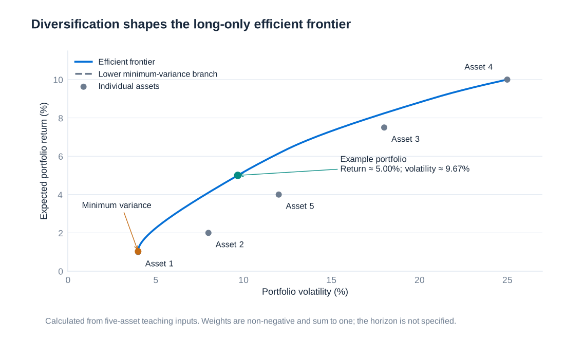
Let be the fraction of portfolio value invested in asset , with , and let denote its return. For fixed weights over the measurement period, portfolio return is . If and , then:
The vector contains the weights and the matrix contains covariances. Its diagonal entries are individual variances. Off-diagonal entries satisfy , where is the return correlation. Portfolio risk is therefore not a simple weighted average of individual volatilities. Diversification depends on how assets move together, and a correlation estimated in calm conditions may not describe a stressed market.
| Asset | Expected return | Volatility | Weight |
|---|---|---|---|
| 1 | 1.00% | 4.00% | 3.10% |
| 2 | 2.00% | 8.00% | 21.48% |
| 3 | 7.50% | 18.00% | 23.77% |
| 4 | 10.00% | 25.00% | 11.52% |
| 5 | 4.00% | 12.00% | 40.13% |
The pairwise correlations are , , , , , , , , and . Correlations are symmetric and each asset has correlation 1 with itself. Converting percentage returns to decimals before multiplying gives the following covariance matrix.
| Asset | 1 | 2 | 3 | 4 | 5 |
|---|---|---|---|---|---|
| 1 | 0.001600 | 0.001600 | 0.001440 | 0.003000 | 0.002400 |
| 2 | 0.001600 | 0.006400 | 0.005760 | 0.006000 | 0.000960 |
| 3 | 0.001440 | 0.005760 | 0.032400 | 0.031500 | 0.003240 |
| 4 | 0.003000 | 0.006000 | 0.031500 | 0.062500 | 0.006000 |
| 5 | 0.002400 | 0.000960 | 0.003240 | 0.006000 | 0.014400 |
For example, . Multiplying the expected returns by their weights gives , approximately 5.00%. The quadratic form gives variance 0.0093482194 and standard deviation 0.0966862, approximately 9.7%. These numbers refer to the same horizon as the inputs. A spreadsheet implementation uses a weighted sum for the mean and matrix multiplication for ; the matrix should be symmetric and positive semidefinite. Rounding its entries too aggressively can distort the result.
Normal quantiles and a portfolio VaR calculation
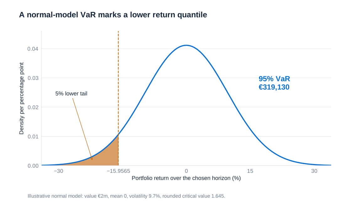
If the vector of asset returns is jointly normal, every fixed linear combination is normal. It is not enough that each asset has an individually normal marginal distribution: the joint dependence structure also matters. Under the joint-normal assumption, . If , then . Approximately 5% of standard-normal observations lie below −1.645 and 5% above 1.645.
The lower 5% portfolio-return quantile is consequently . For initial value and simple return over the chosen horizon, the corresponding normal loss quantile is:
Loss is measured relative to initial value here. A risk system that measures losses relative to expected value would report a different convention. The formula can also produce a negative loss quantile when expected gains dominate the selected threshold; reporting systems sometimes floor VaR at zero, but that convention should be stated rather than silently changing the mathematics.
| Confidence level | Positive quantile, approximately |
|---|---|
| 50% | 0.000 |
| 84.13% | 1.000 |
| 95% | 1.645 |
| 99% | 2.326 |
| 99.90% | 3.090 |
| 99.99% | 3.719 |
Suppose EUR 2 million is invested and the volatility over the risk horizon is taken as the rounded 9.7%. With expected return assumed zero for this separate VaR illustration, the 95% lower return quantile is . The loss threshold is therefore euros, approximately 15.96% of value. This calculation deliberately uses rounded volatility and a zero mean; it does not simultaneously use the five-asset portfolio's 5% expected return.
The horizon cannot be inferred from the final amount. If 9.7% is annual volatility, the result is an annual-horizon calculation; if it describes another horizon, that horizon applies. Scaling volatility by the square root of time requires assumptions about independent increments and stable variance. Fat tails, changing volatility and nonlinear payoffs can make the normal approximation inadequate even when the arithmetic is correct.
Hedging systematic equity risk with index futures
An equity portfolio's systematic exposure can be measured by beta, , where is the market return. A beta of 0.8 means that a one-percentage-point market movement is associated, in the fitted relationship, with approximately a 0.8-percentage-point portfolio movement. It is a sensitivity, not a guarantee that every realised return follows the index. Firm-specific events and changing relationships remain possible.
A manager holding equities can reduce this exposure by selling appropriate stock-index futures. A short futures position gains when the index falls and loses when it rises. Index hedging can be quicker and less costly than selling every holding or hedging each security separately. The relevant index must resemble the portfolio's market exposure: using a DAX-related contract for German equity exposure and an S&P 500-related contract for US exposure are examples of the matching principle, not universal prescriptions.
For a contract with futures price and multiplier , the notional exposure per contract is . A beta-based number of contracts to sell is:
where is current portfolio value and is the desired remaining beta. A positive denotes contracts sold. For market neutrality, . Contract rounding, differences between the cash index and futures price, and basis changes prevent this formula from being a promise of exact protection.
Consider a USD 30 million portfolio with beta 0.8. Its beta-adjusted market exposure is USD 24 million. Using an illustrative E-mini S&P 500 futures level of 8,000 and a USD 50 multiplier gives USD 400,000 notional per contract, so the hedge sells 60 contracts. A 10% index fall implies an approximate USD 2.4 million systematic portfolio loss and an equal gain on the short futures. The combined systematic exposure is million dollars.
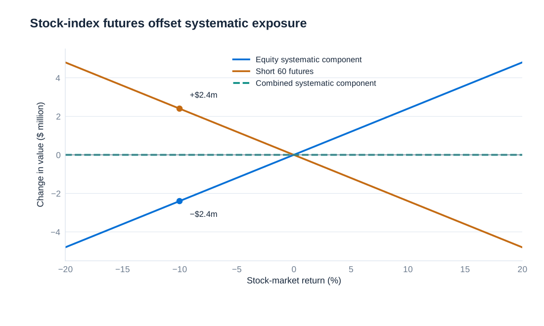
The USD 50 multiplier identifies the particular contract specification used in this example; other contracts have different sizes. A ten-point rise generates a USD 500 gain for the long side and an equal loss for the short side. Cash-settled futures do not require delivery of the underlying shares, and gains and losses are settled through daily variation margin. The familiar quarterly expiry cycle uses March, June, September and December contracts. Holding the hedge requires cash for adverse margin movements even when the combined investment performs as intended.
Market-neutral does not mean risk-free. The portfolio retains idiosyncratic risk, model and beta-estimation risk, basis risk and potentially liquidity risk. Beta can change as positions, prices and business conditions change. A manager must also decide whether to rebalance, roll an expiring contract or tolerate a temporary mismatch. The hedge is successful when it delivers the intended reduction in exposure at an acceptable total cost, not when its derivative leg always reports a profit.
Geometric Brownian motion and positive asset prices
Geometric Brownian motion, or GBM, is a tractable model for a positive asset price. It describes proportional changes rather than adding a normally distributed amount to the price regardless of its level. Its continuous-time specification is:
Here is price or portfolio value at time , is the annualised drift, is annualised volatility, and is a standard Brownian motion. An increment over years satisfies , where . Thus the short-interval approximation is . The random term scales with the square root of time, not time itself.
The exact transition over a finite horizon is:
Equivalently, the log price is normal with mean and variance . The price is lognormal, remains positive and is right-skewed. Finite-horizon simple returns are not exactly normal under this model; normality applies to log returns, while the short-interval proportional-change formula is an approximation. Using the exact exponential update avoids negative simulated prices that a coarse additive approximation could generate.
GBM is useful because its distribution and quantiles can be calculated directly and because it underlies a basic version of option-pricing theory. It remains an assumption. Constant volatility, continuous paths and independent Brownian increments omit volatility clustering, jumps, changing correlations and some features of extreme losses. For real-world risk simulation, drift represents the assumed physical return process. For risk-neutral derivative pricing, the drift is changed consistently with the pricing framework; expected investment return and the risk-free pricing drift should not be interchanged.
Monte Carlo simulation and the interpretation of a risk forecast
Monte Carlo simulation repeatedly draws random inputs and applies the model to generate many possible outcomes. Suppose a portfolio starts at EUR 10,000, with annual drift 9% and volatility 15%, and is projected over five years. A simulation of 10,000 paths can use monthly time steps, , and the exact GBM transition. At each step, every path receives a fresh independent standard-normal draw. The result is a distribution of hypothetical model outcomes, not 10,000 forecasts that the market is expected to follow.
Digital investment services such as Scalable Capital have used distribution-based illustrations to explain possible investment outcomes to clients. The useful feature is the display of uncertainty around a central path rather than a single apparently certain future value. The quality of that communication depends on explaining the return and volatility assumptions and the difference between a model quantile and a promised investment result.
Analytical GBM quantiles provide a direct check on the simulation:
The median corresponds to , whereas the expected value is . These differ because the lognormal distribution is skewed. A middle forecast labelled “50% quantile” is a median, not automatically the mean. The following comparison keeps analytical values separate from the estimates produced by one illustrative 10,000-path simulation.
| Horizon | Analytical 5% quantile | Illustrative simulated 5% quantile | Analytical median | Analytical 95% quantile |
|---|---|---|---|---|
| 1 month | EUR 9,373.84 | EUR 9,361.98 | EUR 10,065.84 | EUR 10,808.92 |
| 1 year | EUR 8,453.72 | EUR 8,470.94 | EUR 10,819.34 | EUR 13,846.92 |
| 3 years | EUR 8,260.54 | EUR 8,293.35 | EUR 12,664.91 | EUR 19,417.61 |
| 5 years | EUR 8,538.92 | EUR 8,550.38 | EUR 14,825.30 | EUR 25,739.73 |
The same illustrative simulation produced a five-year 95% quantile of EUR 25,644.96. Its difference from the analytical value is sampling variation, not a new economic assumption. More simulation paths generally reduce Monte Carlo noise, but do not correct an unsuitable model. A documented implementation should record the parameters, time convention and random seed, and compare simulated moments and quantiles with known results where available.
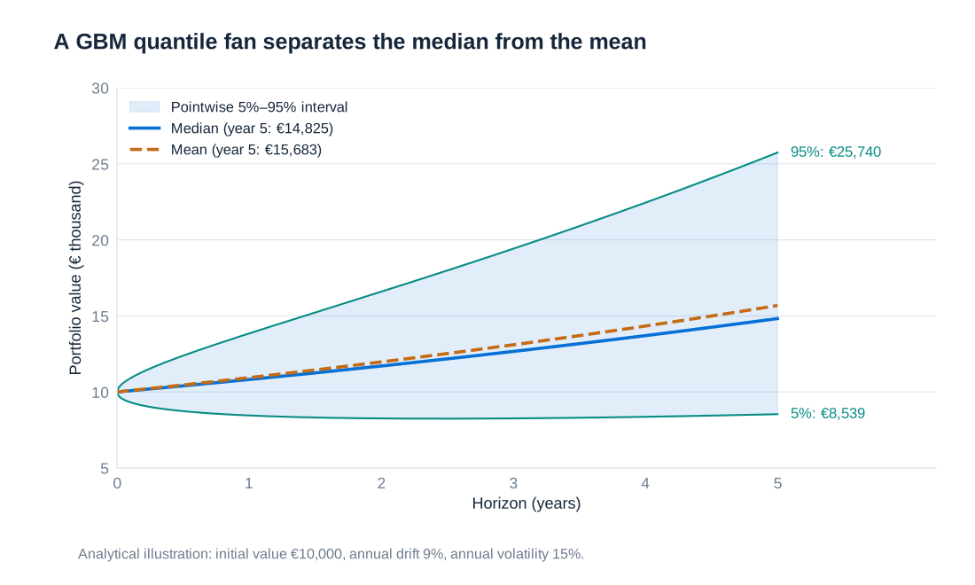
A fan of 5%, 50% and 95% quantiles describes the distribution at each displayed date. It is not a 90% guarantee that an entire path stays inside the band at all intervening dates. Nor is the lowest simulated outcome the maximum possible loss. Distinguishing point-in-time quantiles, path-dependent losses and model uncertainty is essential when communicating risk forecasts to investment clients or decision-makers.
Risk-adjusted performance and incentives
High returns do not by themselves demonstrate skill. A portfolio can earn more because it takes more risk, employs more leverage or accepts an infrequent large loss. Risk-adjusted performance measurement compares reward with the relevant exposure and helps evaluate business units, managers and compensation. The chosen measure must match the decision: total volatility, systematic market risk and capital consumption answer different questions.
Under the capital asset pricing model's assumptions, efficient portfolios combining a risk-free asset and the market portfolio lie on the capital market line:
Here is the risk-free return over the same period, and are the market's expected return and volatility, and is portfolio volatility. The Sharpe ratio measures excess return per unit of total volatility: . With illustrative market return 10%, risk-free return 3% and volatility 20%, it equals . This is an example, not a permanent empirical Sharpe ratio guaranteed by investing in the market.
The security market line instead relates expected return to beta:
It applies in the CAPM to individual securities and portfolios, including inefficient portfolios, because diversifiable risk is not priced in that model. The Treynor ratio divides excess return by beta, . Jensen's alpha measures return above the CAPM benchmark:
Sharpe is appropriate when the investor bears the portfolio's total risk; Treynor and alpha focus on systematic risk and depend on the benchmark model. Treynor becomes difficult to interpret when beta is near zero or negative. Ex-post estimated alpha is uncertain and can reflect an omitted risk factor rather than skill. Comparing ratios also requires consistent horizons, financing assumptions and return definitions.
For a bank business unit, risk-adjusted return on capital, or RAROC, commonly compares risk-adjusted income with allocated economic capital. The numerator should specify the treatment of expected losses, operating costs and taxes; the denominator should identify the capital convention. Comparing RAROC with a required return on capital links performance to shareholder value. Compensation based on this framework can be more informative than a bonus tied only to current profits, but it still requires independent risk measurement, limits, accountability and attention to losses that emerge after the measurement period.
2. Foreign-exchange exposure and corporate hedging
Foreign-exchange risk is the possibility that currency movements change a firm's cash flows, reported financial position or competitive value. The currency printed on an invoice is only the starting point. A business can have substantial currency exposure without signing a contract in that currency, and a hedge that stabilises an accounting number can create a new cash-flow problem. Effective management begins by defining the exposure, the objective and the exchange-rate quotation before selecting an instrument.
Exchange-rate quotations and transaction exposure
Let denote units of home currency required to buy one unit of foreign currency at time . For a euro-based company receiving dollars, is euros per US dollar. A rise in this rate means dollar appreciation against the euro; a fall means dollar depreciation. If a source instead quotes dollars per euro, the economic interpretation of an increase is reversed. The two rates are reciprocals, so their percentage changes are not exactly equal and opposite for large movements.
A fixed foreign-currency receipt due at time has home-currency value . Its sensitivity to the exchange rate is , and a movement changes its value by . This relationship is exact when the amount received remains fixed. A foreign-currency payment has the opposite exposure from the payer's perspective: an appreciating foreign currency raises its home-currency cost. A forecast sale adds uncertainty about the amount and timing of the receipt, not merely the conversion rate.
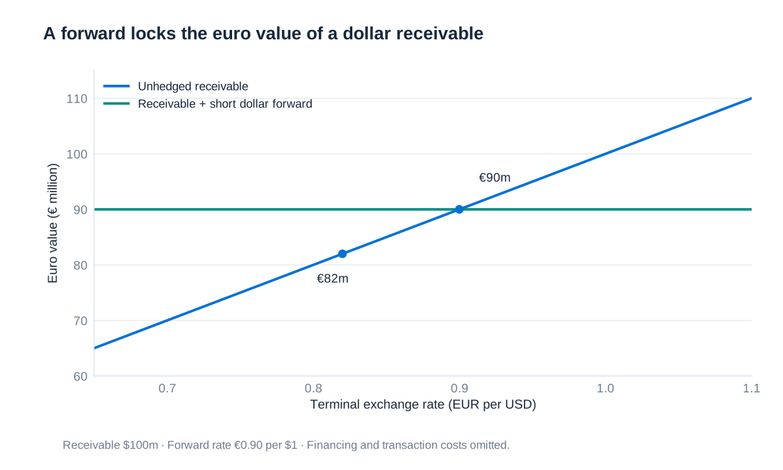
Suppose a German manufacturer plans to sell 1,000 cars in the United States and expects USD 100 million from those sales. At EUR 0.90 per dollar, the expected conversion is EUR 90 million. If the dollar falls to EUR 0.82, the same dollar amount converts to EUR 82 million, a reduction of EUR 8 million. The dollar sales revenue has not changed; its euro value has. Conversely, a euro-based buyer owing USD 100 million benefits from the lower rate. Risk direction must therefore be established from the actual cash flow.
Transaction exposure includes contracted receivables and payables as well as sufficiently identified planned transactions. The distinction matters for hedging. A derivative covering a fixed receivable offsets a known nominal amount. A derivative covering forecast sales can become an unbacked currency position if the sales fail to occur. Netting inflows and outflows in the same currency and period can reduce the amount requiring an external hedge, but netting should respect timing, legal entities and access to the relevant cash.
Operational choices before derivatives
Consider a stylised Porsche example in which the manufacturer produces in Germany, pays its operating costs in euros and sells cars both in the euro area and in the United States. A weaker dollar reduces the euro value of US receipts if dollar prices and quantities remain fixed. One response is to stop serving the US market, avoiding the exposure at the cost of abandoning revenue and strategic opportunities. Another is to raise dollar prices enough to preserve the euro revenue per car.
Passing currency changes to customers does not necessarily remove the business risk. Higher dollar prices can reduce sales when demand is price-sensitive or competitors do not raise their prices. A company may therefore replace exchange-rate risk per unit with quantity risk. Contracts that fix prices for long periods make adjustment slower; strong differentiation or market power can make it easier. Exposure depends on the interaction between currency, prices and volumes.
A natural hedge matches foreign-currency revenue with costs or financing in that currency. Production, procurement, sales activity or research spending in the United States can generate dollar costs against dollar receipts. Dollar borrowing creates dollar interest and principal payments that also offset some inflows. These decisions have consequences beyond currency risk: plant location affects productivity and supply chains, while borrowing affects leverage, maturity structure and credit risk. They should be evaluated as business choices rather than as costless substitutes for derivatives.
Financial hedges, including forwards, futures, options and currency swaps, can then address the residual exposure without moving production. A money-market hedge can create a similar economic offset through borrowing and lending in the relevant currencies. The appropriate combination depends on cash-flow certainty, horizon, market access, transaction costs and the firm's ability to fund collateral or settlement.
Transaction, translation and economic exposure
Transaction exposure focuses on the home-currency value of future receipts and payments. It is often measured over the next quarter or year because contracts and sales forecasts are more identifiable over shorter horizons. Translation exposure concerns the effect of exchange rates on financial statements when foreign-currency balances or the accounts of foreign operations are expressed in the reporting currency. Economic, or operating, exposure concerns the effect of currency movements on the firm's future competitive position and value.
| Exposure | Object being measured | Example | Main difficulty |
|---|---|---|---|
| Transaction | Home-currency cash receipts and payments | A euro-based company expects a fixed dollar receivable | Matching amount and settlement date, especially for forecast transactions |
| Translation | Reported assets, liabilities, equity and results | A foreign subsidiary's net assets are translated into euros | Accounting changes may not generate cash available to fund a hedge |
| Economic or operating | Longer-term cash flows, competitiveness and firm value | A competitor's costs fall when its production currency weakens | Prices, quantities and business responses change together |
The categories can overlap. A foreign subsidiary generates operating cash flows, holds balance-sheet positions and affects the group's competitive strategy. It is still useful to separate the objectives because a hedge designed to stabilise next year's euro earnings may not protect long-term firm value or a regulatory capital ratio. A policy that simply says “hedge currency risk” leaves the most important decision undefined.
Why hedging policies differ across firms
Historical survey evidence from M. Glaum's study of German non-financial corporations illustrates the diversity of practice. The percentages below describe the cited sample rather than current universal frequencies. Most respondents reported flexible hedging, while others used full coverage, a fixed proportion or no hedging. The distinction is economically meaningful: a rule-based hedge stabilises a defined exposure, whereas a flexible policy can incorporate changes in forecasts, costs or management views.
| Policy | Reported share |
|---|---|
| Never hedge | 11% |
| Always hedge 100% | 22% |
| Hedge a fixed percentage | 12% |
| Situational or flexible hedging | 54% |
| Seek additional profit through speculation | 1% |
| Horizon policy | Reported share |
|---|---|
| Three months | 19% |
| Twelve months | 39% |
| Three years | 2% |
| Longer than three years | 2% |
| No fixed rule | 39% |
The horizon percentages sum to 101% because the reported figures are rounded. They should not be rescaled and presented as if more precise information were available. More fundamentally, a five-year hedge can be inappropriate when the quantity of sales five years ahead is highly uncertain. The problem is exposure estimation, even if a sufficiently long-dated derivative can be obtained.
Owners differ in diversification and risk preferences. A family whose wealth is concentrated in one firm may value stable cash flows differently from a globally diversified fund. Managers whose compensation depends on reported earnings may also dislike currency-related earnings surprises. Currency risk can be material for one business and negligible relative to other risks for another. Differences in demand elasticity, price-adjustment frequency, foreign costs and forecasting ability make identical hedge percentages unlikely to suit every firm.
When corporate hedging can create value
In an ideal frictionless capital market, changing the firm's currency payout pattern need not create shareholder value. Investors who can reproduce the hedge themselves at the same cost can choose their own exposure. A globally owned business also has no single currency that represents every shareholder's consumption or liabilities. Stable euro earnings may still be volatile in dollars for a US investor. Hedging is therefore not justified merely by saying that all volatility is undesirable.
Real-world frictions change the argument. Financial distress is costly, and a currency loss can cause a covenant breach, a rating downgrade or forced financing on unattractive terms. Stabilising operating cash flows can help preserve funding for positive-net-present-value investment when external finance is expensive. This is the investment-financing rationale associated with Froot, Scharfstein and Stein: the hedge protects the capacity to undertake valuable projects, not simply the appearance of smooth earnings.
Taxes can also matter when expected tax payments are a convex function of income, although the effect depends on the actual tax system, loss offsets and other circumstances. Firms may execute hedges more cheaply than small shareholders because of scale and market access. Managers and concentrated shareholders may be poorly diversified, creating both reasons to reduce distress and agency concerns about excessive hedging to protect their own positions. The value of a hedge must therefore be assessed against its costs and its effect on the firm's real decisions.
Forwards, options and the mechanics of an offset
A forward fixes today the rate at which currencies will be exchanged at a future date. A company expecting dollars can agree to sell them for euros at maturity. Combining the receipt with the short-dollar forward produces:
With USD 100 million and euros per dollar, the combined amount is EUR 90 million. If the spot rate at receipt is 0.82, the receivable converts to EUR 82 million and the forward contributes EUR 8 million. If the dollar strengthens to 0.98, the receivable converts to EUR 98 million and the forward loses EUR 8 million. The hedge removes the upside and downside around the contracted conversion rate. A derivative loss in the second scenario is the cost of the certainty previously chosen, not proof that the hedge failed.
A foreign-currency payable requires the opposite direction: a forward purchase of foreign currency. Its payoff is , which offsets the increase in the unhedged payment . A call option on the foreign currency offers the right to buy at a strike rate and therefore places a ceiling on the payment, while preserving the benefit of a cheaper foreign currency. The option buyer pays a premium for this asymmetry. A foreign-currency receivable can instead be protected with a put on that currency.
Futures are standardised and settled through daily margining; forwards are typically tailored over-the-counter agreements whose collateral terms depend on the contract. Both can create funding needs before the commercial exposure settles. Options have a different pattern of premiums and potential margin requirements depending on whether the company buys or sells them. A hedge policy should distinguish an option purchase that limits downside from writing options that may add exposures the business never intended to take.
Forward pricing, money-market hedges and cost of carry
A forward rate is not generally equal to today's spot rate and is not simply a prediction of the future spot rate. Under a simplified no-arbitrage framework with continuous compounding, home interest rate , foreign interest rate and maturity years, covered interest parity gives:
The quotation remains home currency per foreign currency. The difference between interest rates determines the forward adjustment because holding foreign currency has a foreign-currency financing or investment return. The formula assumes consistent borrowing and lending opportunities and abstracts from transaction costs, credit effects and cross-currency basis. Those assumptions explain the economic benchmark; observed quotes may reflect additional market frictions.
A money-market hedge reproduces the same logic. To hedge a foreign-currency receipt at , borrow its foreign-currency present value, convert that amount into home currency today and invest the home proceeds until . The actual receipt repays the foreign loan. Using the stated continuous rates, the home proceeds are . The strategy uses borrowing capacity and changes the balance sheet, so an economic equivalence does not make every implementation equally convenient.
The related cost-of-carry principle applies to a non-income-paying investment asset. If it can be bought for and financed at continuously compounded rate , a simple benchmark is . For a spot value of EUR 80, an annual financing rate of 5% and delivery in six months, euros. This example excludes asset income, storage costs and convenience benefits. It must not be confused with the currency formula, in which the foreign interest rate plays the role of a yield on the asset being held.
Translation exposure and the liquidity cost of hedging
A foreign operation may keep its accounts in a functional currency different from the group's presentation currency. Translating those accounts can change reported assets, liabilities and equity even when no sale or cash transfer occurs. If dollar-denominated net assets lose euro value as the dollar weakens, the group's reported equity can decline. The resulting effect on leverage or a covenant can matter even if the subsidiary's local operations are unchanged.
Under IAS 21, ordinary translation of a foreign operation into a different presentation currency generally places resulting exchange differences in other comprehensive income, or OCI, subject to the standard's conditions. This is distinct from remeasuring a foreign-currency monetary receivable in the entity's own functional currency, where exchange differences generally enter profit or loss. Treating every foreign-currency accounting change as the same type of translation exposure obscures this distinction.
Hedging a net investment can create a mismatch between realised cash and unrealised accounting gains. Suppose dollar appreciation raises the euro-translated value of a subsidiary's net assets by EUR 1 billion. A short-dollar hedge intended to offset that rise may require cash settlement or collateral even though the subsidiary has not distributed any cash. The accounting offset can be effective while the parent faces a liquidity demand. This is one reason some translation exposures remain unhedged.
It is too strong to say that translation exposure never affects earnings or is never hedged. Disposals, transaction balances, different functional-currency circumstances and designated hedging relationships can change the accounting treatment. More importantly, a firm may wish to protect a capital ratio or debt capacity rather than current profit. The decision should identify the relevant objective and the cash needed to support the hedge through adverse currency movements.
Why matching foreign assets and liabilities does not fix every ratio
Borrowing in the currency of foreign assets can reduce the sensitivity of net assets. If dollar assets and dollar liabilities are equal in amount, a change in their common euro conversion rate leaves their net contribution to equity approximately unchanged. Yet the gross balance-sheet amounts can still expand. With equity held constant, an increase in total assets raises assets-to-equity leverage and reduces an equity-to-assets capital ratio.
This distinction also applies to the regulatory leverage ratio. In that context the numerator is defined Tier 1 capital and the denominator is a regulatory exposure measure, not simply accounting assets. A stronger foreign currency can increase the denominator even when matched assets and liabilities offset economically. It is therefore essential to state whether “higher leverage” means a higher assets-to-capital multiple or a lower capital-to-exposure ratio.
A historical example is Deutsche Bank's first-quarter 2015 reporting: leverage exposure was EUR 1,549 billion at 31 March 2015, an increase of EUR 104 billion from year-end 2014, attributed almost entirely to exchange-rate movements. The figures illustrate how currency translation can affect a regulated denominator. They do not show that the bank incurred a EUR 104 billion loss, and they should not be interpreted as a current balance-sheet measure.
Foreign-currency instruments and accounting measurement
Accounting classification determines how price changes and exchange differences reach the statements, but banking-book and trading-book labels do not alone resolve every measurement question. Under IFRS, an instrument held for trading is normally measured at fair value through profit or loss. Its home-currency value can change because of the instrument's foreign-currency price and because of the exchange rate. Both components matter even when the issuer's contractual payment remains unchanged.
A foreign-currency government bond qualifying for amortised-cost treatment under IFRS 9 is different. A pure change in market yields does not by itself remeasure its carrying amount to the new market price. Effective-interest accounting, expected-credit-loss requirements and foreign-currency remeasurement still apply. As a monetary item, it is normally translated at the closing rate under IAS 21, with exchange differences generally recognised in profit or loss, subject to specified exceptions. “Held to maturity” is therefore not a reason to ignore exchange-rate movements.
German bank accounts under the HGB require a separate analysis. Section 340e(3) requires financial instruments in the trading portfolio to be measured at fair value less a risk deduction. This is different from a blanket rule that recognises all losses but never unrealised gains. For other assets, classification and the relevant valuation provisions matter. Currency translation must then be considered separately: section 256a provides a closing-spot-rate rule, while section 340h contains bank-specific provisions for positions specially covered in the same currency.
A general statement that a German bank's long-term foreign bond is unaffected by exchange-rate changes unless it suffers permanent impairment is consequently unreliable. Asset valuation, currency conversion, maturity and currency matching are separate parts of the analysis. The accounting result should also be separated from the economic exposure: a stable carrying amount does not mean the position could be sold at that amount or that its future cash flows are riskless in home currency.
Accounting references: IAS 21; HGB section 340e; HGB section 256a; HGB section 340h.
Economic exposure and operational flexibility
Economic exposure concerns changes in future cash flows and firm value caused by currency movements, including effects that are not attached to a booked receivable or payable. A European motorcycle producer can face yen exposure even if it sells few motorcycles in Japan and invoices almost nothing in yen. Japanese competitors pay important costs in yen. Yen depreciation can improve their ability to reduce prices abroad, putting pressure on the European producer's volumes or margins. Yen appreciation can reverse part of that competitive advantage.
The BMW motorcycle example illustrates this mechanism across changing competitive conditions: a largely domestic cost base does not eliminate exposure to the currencies of foreign competitors. A full historical account would also consider technology, product quality and market strategy, so exchange rates should not be presented as the sole explanation of decades of competitive performance. The essential distinction is between direct currency cash flows and indirect competitive sensitivity.
Operational hedging changes the structure of the business. Production and labour costs can be located closer to the markets generating revenue. Procurement can shift toward suppliers in the relevant currency, and shorter sourcing contracts may preserve flexibility. Maintaining the ability to move production between locations creates a real option: management can respond to future conditions instead of committing irrevocably to one cost structure. That flexibility has costs, including spare capacity and organisational complexity.
Financing can also be matched to durable operating inflows through foreign-currency debt or currency swaps. However, a financial derivative is usually tied to a fixed nominal amount and horizon, whereas economic exposure depends on changing prices, quantities and competitive responses. A large hedge based on a weak long-range sales forecast can increase rather than reduce risk. Scenario analysis should therefore examine the business response, not just mechanically translate a fixed cash-flow forecast at different rates.
Transfer restrictions and exchange-rate regime changes
Currency convertibility and the ability to transfer money are separate from the exchange rate itself. A subsidiary can earn profits abroad while capital controls, administrative restrictions or political decisions prevent distribution to the parent. Concerns reported about the transfer of profits from China illustrate this distinction. A derivative that fixes the conversion rate does not necessarily provide legal access to the underlying cash or permission to remit it.
Exchange-rate regimes can also change abruptly. The Swiss franc's history illustrates both safe-haven demand during financial stress and the risk of assuming that an official exchange-rate policy will persist. The Swiss National Bank's removal of its minimum exchange rate against the euro in January 2015 caused a sharp repricing. A period of low observed volatility under a policy regime may therefore understate the losses possible when that regime changes.
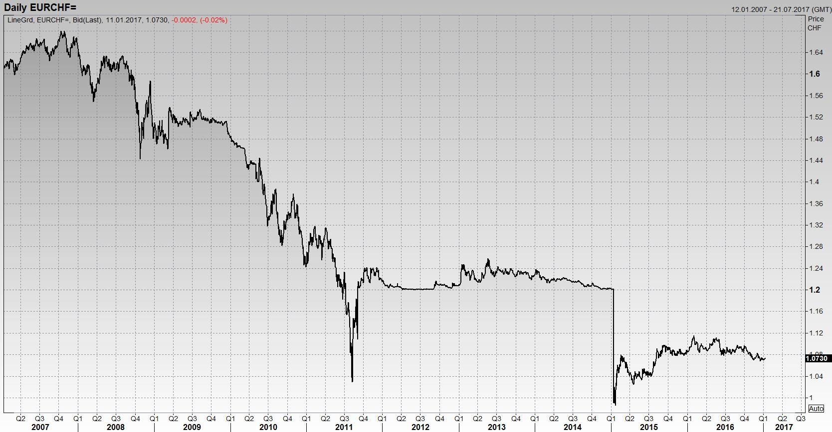
These risks call for controls beyond a statistical estimate based on recent returns. Treasury should consider currency access, legal entities, settlement channels and the possibility that markets become discontinuous. Liquidity planning must allow for adverse collateral calls or the need to obtain currency when ordinary dealing conditions are unavailable.
Historical source: SNB, discontinuation of the minimum exchange rate, 15 January 2015.
The Lufthansa aircraft-purchase decision
The Lufthansa case concerns a decision made in January 1985 to purchase 20 Boeing 737 aircraft for USD 500 million, payable approximately one year later. The dollar had appreciated substantially against the Deutsche mark. The central question was how to manage the mark cost of a fixed dollar payment while preserving the airline's ability to finance its aircraft. A view that the dollar looked expensive was not a guarantee that it would decline before settlement.
For a transparent numerical comparison, let be the terminal exchange rate in Deutsche marks per dollar, assume a forward rate of DM 3.2 per dollar, and compare four strategies: no hedge, full forward cover, half forward cover and a call option on dollars. For the option example, assume a strike of DM 3.2 and a total premium of DM 100 million. The premium is an explicit illustrative input; its financing cost is ignored so that the payoff comparison remains clear.
With million dollars, the unhedged payment is . A full forward fixes it at million marks. A half hedge fixes USD 250 million at 3.2 and buys the remaining USD 250 million at spot. A dollar call permits purchase at the lower of the spot rate and strike, but requires the premium. In DM billions, the four total costs are:
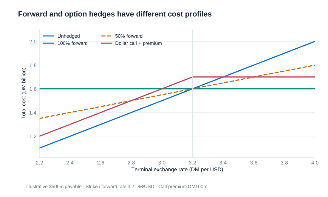
| Terminal DM per USD | Unhedged | Full forward | Half forward | Call option including premium |
|---|---|---|---|---|
| 2.2 | 1.10 | 1.60 | 1.35 | 1.20 |
| 2.4 | 1.20 | 1.60 | 1.40 | 1.30 |
| 2.6 | 1.30 | 1.60 | 1.45 | 1.40 |
| 2.8 | 1.40 | 1.60 | 1.50 | 1.50 |
| 3.0 | 1.50 | 1.60 | 1.55 | 1.60 |
| 3.2 | 1.60 | 1.60 | 1.60 | 1.70 |
| 3.4 | 1.70 | 1.60 | 1.65 | 1.70 |
| 3.6 | 1.80 | 1.60 | 1.70 | 1.70 |
| 3.8 | 1.90 | 1.60 | 1.75 | 1.70 |
| 4.0 | 2.00 | 1.60 | 1.80 | 1.70 |
The full forward removes exchange-rate uncertainty in this simplified calculation. The half hedge leaves half the slope of the unhedged cost curve. The option caps the total at DM 1.7 billion while retaining gains from a cheaper dollar, after allowing for its premium. The dollar protection is a call on dollars, equivalently involving a put on marks under the reciprocal currency description; calling it a dollar put would reverse the protection.
Ex-ante protection and ex-post regret
The dollar subsequently fell from approximately DM 3.2 to DM 2.2. Buying USD 500 million at the new spot rate would cost DM 1.1 billion instead of DM 1.6 billion. A half forward hedge at 3.2 generates a derivative loss of million marks relative to spot, leaving a combined cost of DM 1.35 billion. The hedge gives up half the favourable currency movement in return for having protected half the payment against an unfavourable movement.
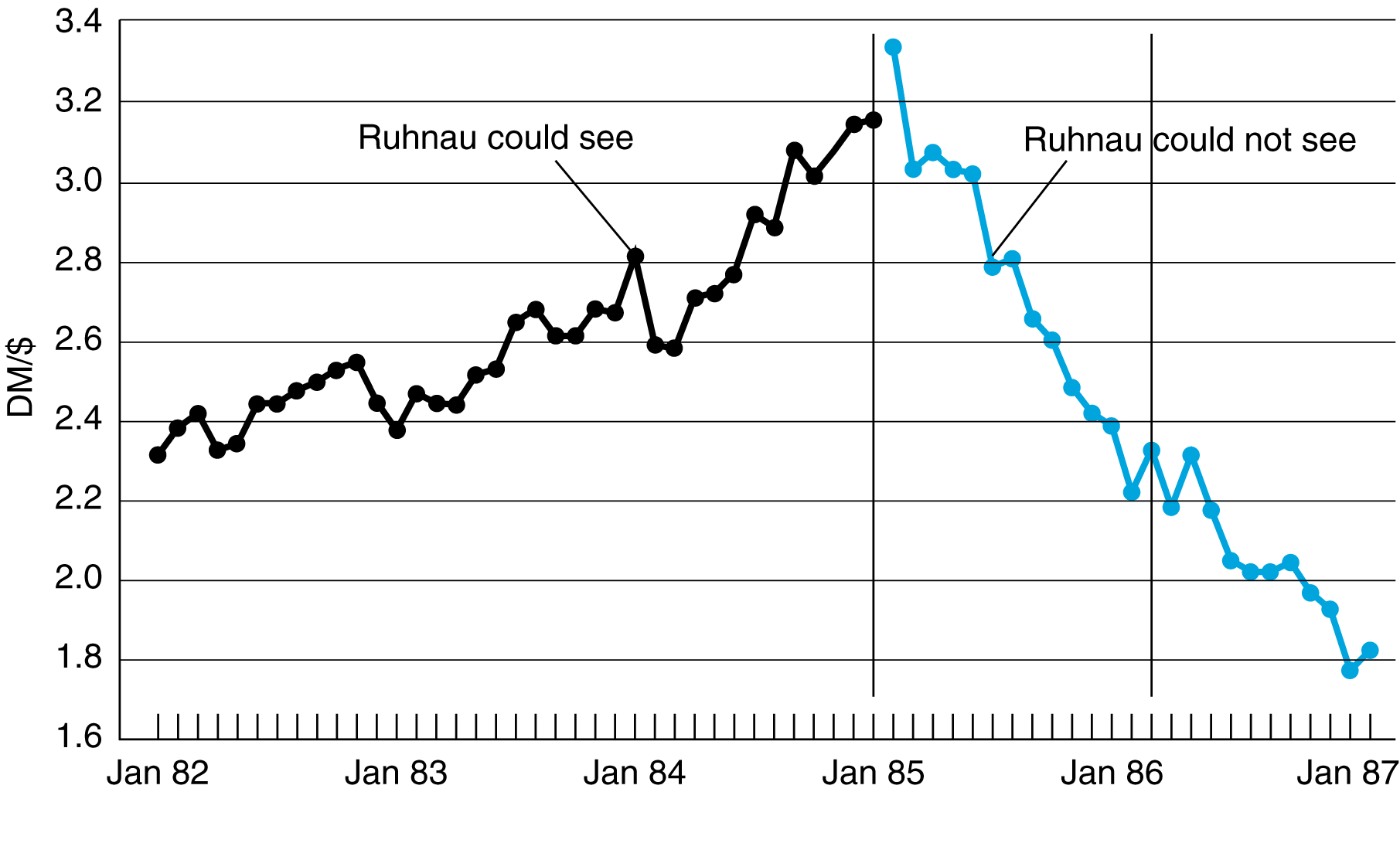
Criticism based only on the realised forward loss ignores the decision's original purpose. Had the dollar risen to DM 4, the half hedge would have gained DM 200 million and reduced the DM 2 billion spot cost to DM 1.8 billion. The appropriate ex-ante assessment asks whether the chosen exposure, certainty and cost suited the airline's objectives using information available at the time. The strategy need not be optimal merely because it was a hedge, but hindsight about the direction of the dollar is not a sufficient performance criterion.
The case also highlights governance. Management and the supervisory board need agreement on whether the objective is to fix an investment budget, protect cash flow, stabilise accounting earnings or express a currency view. A partial hedge can be sensible under a defined policy, but looks arbitrary when no one can explain why that proportion was chosen. Clear reporting should distinguish the derivative result, the underlying purchase cost and the combined outcome.
Why the aircraft and the hedge can affect earnings differently
Buying an aircraft normally exchanges cash for a non-financial asset recognised at its acquisition cost. In a simplified initial-recognition example, that transaction does not immediately produce an operating profit or loss. A cheaper aircraft leaves more cash and a lower recorded asset cost; it does not necessarily create a current-period accounting gain equal to the currency saving. Depreciation and later measurement effects occur subsequently.
| Item | Before purchase | Purchase at DM 4 per USD | Purchase at DM 2 per USD |
|---|---|---|---|
| Cash | 2 | 0 | 1 |
| New aircraft | 0 | 2 | 1 |
| Other assets | 8 | 8 | 8 |
| Total assets | 10 | 10 | 10 |
| Debt | 5 | 5 | 5 |
| Equity | 5 | 5 | 5 |
This balance sheet deliberately excludes derivative settlement and later depreciation. A 50% forward hedge of USD 500 million at 3.2 produces a DM 0.2 billion gain if the terminal rate is 4, and a DM 0.3 billion loss if it is 2. Without an accounting treatment that appropriately aligns the hedge with the exposure, the derivative result can enter earnings while the purchase-price difference is reflected in the aircraft's carrying amount. The economic offset and the timing of reported earnings can therefore differ.
Modern hedge accounting addresses specified mismatches when its designation, documentation and effectiveness requirements are met; it is not automatic simply because management calls a transaction a hedge. Nor should a historical case be used to claim that no form of hedge accounting existed anywhere in 1986. The durable lesson is to analyse both economic protection and accounting presentation before entering the transaction.
Putting the currency policy together
A corporate currency policy starts with the business decisions that generate risk: markets served, locations of operations and currencies used for pricing and financing. It then defines which transaction, translation and economic exposures matter, how confidently they can be forecast, the horizons to be covered and the permitted hedge percentages. The instrument choice follows these objectives rather than preceding them.
Limits can be expressed through nominal exposures, Value at Risk, Cash Flow at Risk or Earnings at Risk, depending on the quantity the firm seeks to protect. Operational hedges, foreign-currency borrowing, money-market transactions and derivatives should be considered together. Treasury also needs a process for exposure updates, collateral funding, counterparty limits and exceptions. A policy that reduces reported currency volatility while creating an unmanageable cash requirement has solved the wrong problem.
Transaction exposure is often the most straightforward to hedge because its amount and date can be identified. Translation exposure requires special attention to the difference between accounting gains and available cash. Economic exposure is often substantial but less directly matched by fixed-notional derivatives. The overall objective is a coherent relationship between the firm's operations, financial capacity and chosen currency risk, with the combined position understandable to those responsible for oversight.
3. Commodity Price Risk and Minimum-Variance Hedging
Commodity risk arises because the prices, quantities and delivery conditions of physical inputs and outputs change. An airline purchases fuel, an oil producer sells petroleum, and a manufacturer may be exposed on both sides through energy costs and product prices. Their exposure is the effect on the whole business, not simply the movement of one quoted commodity price. A derivative can offset that exposure, but its effectiveness depends on matching the commodity, quantity, maturity and cash-flow timing. Price protection can therefore coexist with basis risk, counterparty risk or a serious demand for cash.
Trading rewards, operating exposures and the purpose of a hedge
In December 2023, reporting on Goldman Sachs trader Ed Emerson put his three-year compensation near USD 100 million, illustrating potential commodity-trading rewards. Such examples must be distinguished from the objective of a corporate hedging programme. A trader may earn money by supplying liquidity, intermediating client transactions or deliberately accepting market exposure. An operating company normally hedges to stabilise an input cost, selling price, cash flow or balance-sheet value. The fact that a derivative loses money does not establish that the hedge failed: that loss may accompany an economically valuable gain in the underlying business.
A producer expecting to sell a known quantity is adversely exposed to falling prices; a consumer expecting to purchase it is adversely exposed to rising prices. The producer generally needs a short price hedge and the consumer a long price hedge. This directional rule applies to the specified exposure, not automatically to the company's name or industry. An oil distributor that has promised fixed-price deliveries but has not yet acquired the oil is exposed to rising acquisition costs, even though it will ultimately be selling the commodity to customers.
The risk-management objective should specify the quantity, delivery location, quality, currency and dates of the exposure, together with the loss measure and horizon. Hedging a price per barrel does not by itself hedge an uncertain number of barrels. Likewise, a crude-oil contract does not exactly hedge jet fuel, which includes refining and product-specific market effects. These distinctions explain why an apparently simple one-for-one hedge can leave substantial risk.
Forward contracts, futures and settlement obligations
A long forward commits its holder to buy a specified underlying at a delivery price agreed today; a short forward commits its holder to sell. Let be the agreement date, the delivery date, the spot price at delivery and the agreed delivery price per unit. Ignoring costs and default, the terminal economic payoffs are
For physical delivery, the long party pays and receives an asset worth . Cash settlement pays the economically equivalent difference when the contract specifies it. These are linear payoffs: a one-unit increase in the terminal price raises the long payoff by one unit and lowers the short payoff by one unit. For units of the underlying, multiply the payoff by .
A forward agreed at the current fair delivery price normally has zero initial market value. Zero initial value does not mean zero risk, zero future liability or unlimited access to funding. A contract agreed away from the fair price has a nonzero value, and collateral arrangements can require cash before maturity. Bilateral forwards also expose each party to the possibility that an in-the-money counterparty fails to perform.
Exchange-traded futures are standardised contracts supported by a clearing and margin system. Initial margin is a performance deposit; variation margin transfers gains and losses as the contract is marked to market. The clearing structure substantially reduces bilateral counterparty exposure, but it does not eliminate every clearing-member, operational, liquidity or extreme default risk. Futures may end in physical delivery or cash settlement. Closing a position before expiry requires an offsetting trade in the relevant contract, not merely a decision to stop recognising its value.
| Feature | Forward | Futures |
|---|---|---|
| Contract terms | Usually negotiated bilaterally | Standardised by the trading venue |
| Initial value and funding | Normally zero fair value at inception; collateral may be required | Initial margin is posted |
| Settlement during the contract | Depends on collateral and contractual arrangements | Variation margin settles marked-to-market gains and losses |
| Principal risk-management consequence | Counterparty exposure and contractual collateral terms matter | Immediate cash requirements can arise despite an economically offsetting exposure |
How a matched forward fixes a purchase cost
Suppose a consumer must buy one unit at and enters a long forward with currency units. The physical purchase costs , while the forward produces . The net cost after the hedge is therefore
If the price rises to 100, the physical cost is 100 and the derivative gain is 20. If the price falls to 60, the physical cost is 60 and the derivative loss is 20. Both cases give a net cost of 80. Evaluating only the derivative in the second case would miss the offsetting saving on the actual purchase. A producer selling one unit would instead combine sale revenue with a short forward, giving .
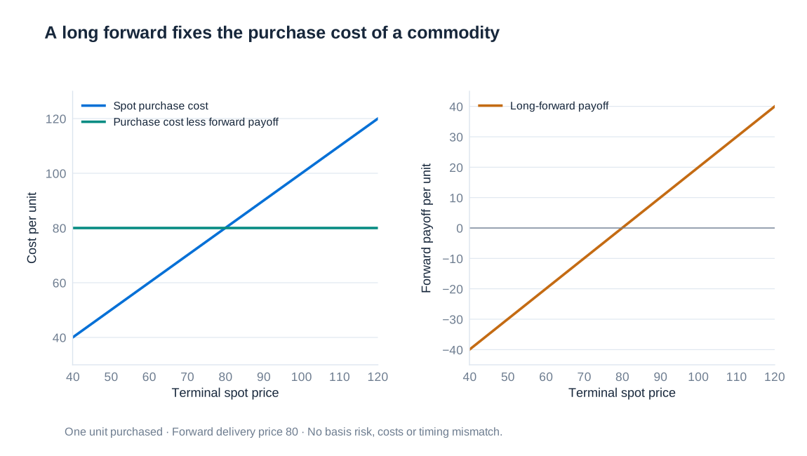
The cancellation requires the purchase and hedge to concern the same underlying, quantity and date and assumes performance by the counterparties. A similar example is a payment of USD 1 million due in three months hedged by a three-month forward that supplies exactly that dollar amount. The exchange-rate exposure of that payment can be removed, although funding, credit and operational risks remain. In a commodity business these matching conditions are often harder to achieve.
Cash-and-carry pricing and its assumptions
For a freely tradable asset that pays no income and has no storage costs, spot and forward prices are linked by financing. Let be the current spot price, the fair forward delivery price, a continuously compounded financing rate per year and the remaining time in years. Buying the asset today and financing it until delivery costs at . Equivalently, a fair long forward plus an investment that grows to the delivery payment produces the same terminal asset. No arbitrage therefore requires
If a forward price were above this financing-adjusted spot price, an investor able to borrow, purchase and store the asset could sell it forward and lock in a difference. The reverse trade requires the ability to short or otherwise obtain the underlying. Transaction costs, credit limits and restrictions on short selling can therefore create bounds rather than an exact relationship in practice.
For example, with a spot price of EUR 80, a continuously compounded annual financing rate of 5% and six months to delivery, the no-income, no-storage calculation is , or approximately EUR 82.03. The difference from the spot price is financing compensation, not automatically a forecast that the future spot price will rise by that amount. Forward prices and expected future spot prices need not coincide because risk premia and other economic forces can matter.
Valuing an existing forward before maturity
The delivery price of an existing contract remains fixed while the fair delivery price for new contracts changes. Suppose an earlier long forward has delivery price . At a later date , an opposite short forward with the same underlying and maturity can be entered at the new fair price . At maturity, the physical obligations offset and the combined payoff is . Under the simple deterministic-rate assumptions, the current value of the original long forward is
If the original delivery price was USD 10 and the new forward price is USD 11, the offset locks in USD 1 per unit at maturity. Its value today is the discounted dollar, not automatically exactly USD 1. The offset removes the price exposure but does not necessarily terminate both contracts or remove their counterparty and collateral obligations. Close-out and netting arrangements determine the contractual result.
Changes in forward prices are consequently a useful approximation to changes in forward value when discounting effects over the interval are small. Futures variation margin, by contrast, is paid or received during the contract's life. Under deterministic interest rates and otherwise identical terms, standard forward and futures prices coincide; with stochastic rates, the relationship between settlement cash flows and rates can produce a difference. The timing of gains and losses is economically relevant even when terminal price exposure appears similar.
Storage costs, convenience yield and the forward curve
Physical inventory can be costly to finance, insure and store, but possessing it can also provide an operating benefit. A refinery with available crude can keep producing during a supply disruption; a firm without inventory may miss a sale or interrupt production. Convenience yield represents this noncash benefit of holding the physical commodity. With proportional storage costs and convenience yield , both expressed as annual continuous rates, a common cost-of-carry representation is
Financing and storage tend to raise the forward price relative to spot, while convenience yield tends to lower it. Contango commonly describes a forward price above spot or an upward-sloping curve across maturities; backwardation describes the opposite configuration. These related usages should be stated clearly. A high convenience yield can support backwardation despite positive financing and storage costs. As a deliverable contract reaches maturity, its price converges to the corresponding spot delivery value under the contract's delivery and settlement rules.
The formula is most informative when the underlying inventory and arbitrage assumptions are credible. Electricity is difficult to store economically at large scale, agricultural goods have seasonality and deterioration, and livestock involve biological production and maintenance. Location, quality and transport constraints further segment markets. Spot and deferred prices can consequently respond differently to the same news. That does not mean that the markets are literally unrelated; it means that a simple immediate storage trade may not enforce a tight price link.
For positive observed prices, an implied convenience yield can always be calculated as . If this unknown is chosen solely to fit the observed forward price, however, the equation becomes a decomposition rather than an independent prediction. A collapse in current oil demand can depress nearby prices more than deferred prices as inventories accumulate and storage becomes scarce. The change in curve shape is then as important to a rolling hedge as the change in the overall price level.
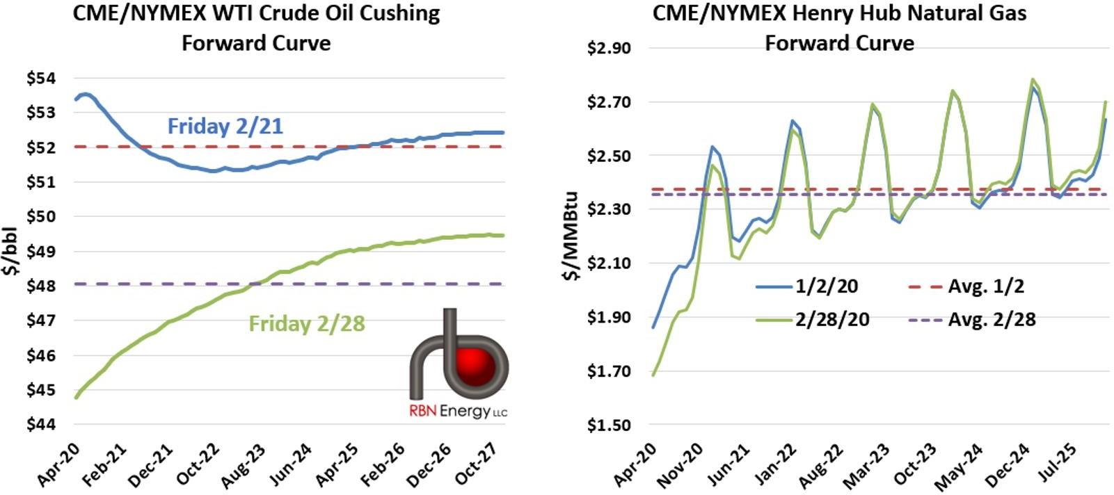
The February 2020 oil-curve comparison illustrates this distinction: nearby and deferred WTI prices both moved, but the size of the decline depended on the delivery month. Comparing entire curves reveals changes in term structure that a single spot-price observation would conceal. These are dated market observations, not a prediction of how every future demand shock must affect the curve.
Basis risk and the minimum-variance hedge
A cross-hedge uses an instrument that is related to, but not identical with, the exposure. Hedging jet fuel using crude-oil futures is an example: the jet-fuel bill and crude futures usually respond to common energy factors but also have separate influences. A hedge can also have maturity basis risk when short-dated contracts are rolled against a long-dated exposure. The relevant relationship is between changes over the actual risk horizon, not simply between long-run price levels.
Let be the unhedged change in the value of the business exposure, in currency, and let be the profit on one long futures contract over the same interval, also in currency. Let be the signed number of contracts: positive means long and negative means short. The hedged value change and its variance are
where , and . Differentiating with respect to gives . If the hedge contract has positive variance, the unique minimum is
where is the correlation of exposure changes and long-contract profits. The minus sign makes the position offset the exposure. A long inventory position generally has positive covariance with a long commodity future, requiring a short hedge. A future purchase cost enters business value with a negative sign; its adverse exposure generally calls for a long hedge. Defining the exposure as a cost instead of value is possible, but then the hedge payoff must be subtracted rather than added.
Contract size, regression estimation and remaining risk
If the exposure is units of inventory at spot price and each futures contract covers units with futures price , then and . The optimal signed number is
This distinguishes a dimensionless price hedge ratio from an actual contract count. For an illustrative inventory of 10,000 units, a contract size of 100 units, correlation 0.8 and a spot-change standard deviation 1.25 times the futures-change standard deviation, the price hedge ratio is . The optimal position is therefore contracts. Rounding, transaction costs and trading limits can make the feasible position differ from the continuous optimum.
Regressing on an intercept and estimates the slope . This is the positive hedge-size coefficient when covariance is positive; the signed inventory hedge is its negative after quantity conversion. The intercept captures an average change and does not itself reduce variance. Estimates should use observations relevant to the intended horizon and be checked for changes in market conditions rather than treated as permanent constants.
Substituting the optimal hedge into the variance expression gives
With a single regressor and an intercept, the regression's equals and measures the fraction of in-sample variance eliminated. Correlation 0.5 removes only 25% of variance; zero correlation offers no variance reduction. Perfect positive or negative correlation permits zero residual variance in this ideal linear model if either hedge direction is available. At correlation 0.7, 51% of the original variance remains and residual standard deviation is approximately 71.41% of its original level.
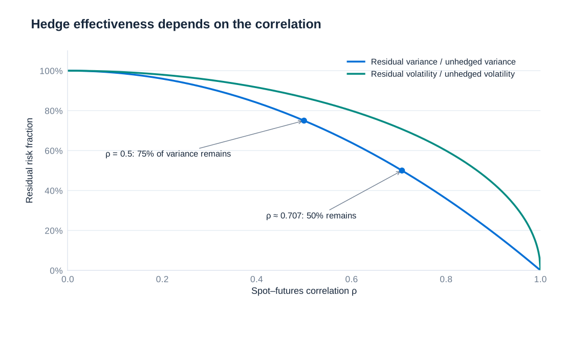
If , as in an illustrative single-stock hedge using index futures, half the variance remains but the remaining standard deviation is , or about 70.7%, not 50%. This distinction is also essential when assessing commodity hedges. Variance efficiency measures a particular price-risk objective; it does not measure the ability to finance margin calls or guarantee that an estimated relationship will hold during a crisis.
When the underlying business disappears: Lufthansa in 2020
A forecast purchase is not the same as an unconditional obligation. The pandemic-related collapse in aviation activity reduced Lufthansa's fuel and currency needs, leaving some previously designated hedges without the forecast transactions they had been intended to offset. Falling fuel prices could then generate derivative losses without a matching saving on fuel that was no longer purchased. An excessive hedge became a separate open exposure.
Lufthansa's 2020 reporting identified EUR 758 million of realised fuel-hedge expenses and EUR 28 million of realised foreign-currency hedge earnings on expired stand-alone derivatives, a net result of EUR −730 million. These figures concern that specified category of derivatives, not the airline's total annual loss or its entire hedging result. The lesson is that volume forecasts, contractual commitments and hedge quantities must be reviewed together. A decision about whether to retain, reduce or close an overhedge also needs the resulting market-value and cash consequences.
Primary source: Lufthansa Annual Report 2020, page 213.
Metallgesellschaft: long-term promises and short-term cash demands
The Frankfurt-based industrial group Metallgesellschaft's oil-related crisis developed in 1993–94 and led to an emergency recapitalisation of the German parent company, rather than a simple completed bankruptcy. The core economic problem involved long-term fixed-price petroleum delivery contracts and large positions in short-term derivatives. The crisis combined price exposure, maturity mismatch, funding requirements and weaknesses in oversight; it cannot be understood by looking only at the final payoff of one futures contract.
A simplified delivery commitment makes the direction clear. If a distributor promises one barrel every month for ten years at a fixed selling price, it has committed to 120 future barrels. Higher purchase prices would reduce its delivery margin. Long oil futures can therefore offset the adverse price direction. But holding near-term futures for all 120 barrels concentrates exposure at the front of the curve, whereas the physical deliveries occur over 120 separate months. Short-term contracts must be rolled and adjusted as deliveries occur.
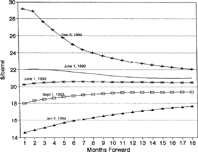
When oil prices fell and the curve moved toward contango, long near-term futures generated losses that demanded immediate cash. Fixed-price customer sales could become more valuable because oil could eventually be purchased more cheaply, but those benefits were spread across future deliveries and were not equivalent to cash available for today's margin call. Different maturities also moved by different amounts, so an economically offsetting direction did not imply an equal offset in present value.
Rolling introduces another mismatch. A long position is closed in the expiring contract and reopened further out. In contango, the new contract may be more expensive than the old one, changing the economics of maintaining exposure. This difference is not necessarily an immediate payment of the whole futures notional: futures are margined contracts. Nevertheless, the evolution of prices, repeated settlements and financing of collateral determine the realised cash-flow path. A hedge that requires funding the company cannot obtain may be impossible to maintain.
Historical analysis: Frankel and Palmer, Federal Reserve International Finance Discussion Paper 560 (1996).
Evaluating hedge size and the complete risk budget
Historical regression estimates associated with the Metallgesellschaft debate illustrate why matching total barrels one-for-one need not minimise variance. The table relates changes in longer-dated futures prices to changes in the nearest one-month futures price over 1990–1992. The slope estimates below one indicate that a unit change in the near-term price was associated with a smaller change in the longer-dated contract; the relationship also varied by product and maturity.
| Contract maturity | Heating oil: slope | Heating oil: R² | Gasoline: slope | Gasoline: R² |
|---|---|---|---|---|
| Two months | 0.735 | 0.84 | 0.740 | 0.80 |
| Three months | 0.625 | 0.79 | 0.650 | 0.75 |
| Six months | 0.513 | 0.80 | 0.562 | 0.76 |
| Nine months | 0.492 | 0.79 | 0.520 | 0.72 |
For example, the six-month heating-oil slope of 0.513 implies a smaller offsetting near-term price exposure than a one-for-one position, under that regression's units and assumptions. Its of 0.80 implies 20% residual variance and about 44.72% residual standard deviation in the fitted single-factor model. These short-maturity historical estimates do not by themselves determine a ten-year delivery programme's optimal hedge. They demonstrate the need to estimate the relevant price relationship rather than assume equal sensitivities.
A hedge also needs clear responsibility for monitoring positions, approving exceptions and arranging collateral before a stressed market closes access to finance. A complete hedge policy combines exposure measurement, a defensible contract size, stress tests of curve changes and volume disruption, and a funding plan for adverse margin paths. Long-term delivery optionality and customer credit risk require separate analysis. Minimum variance is one useful objective, but management may instead need to protect minimum cash balances or avoid a severe funding shortfall. Those objectives can justify a hedge smaller than the unconstrained variance optimum, a different maturity structure or a different instrument.
4. Interest Rate Risk, Duration and Banking-Book Exposure
Interest rates influence both the present value of promised cash flows and the income earned when money is reinvested or funding is renewed. A fixed-rate bond can lose market value when yields rise even though its contractual payments have not changed. A saver rolling short-term deposits can instead be harmed by falling future rates, while a bank faces the combined repricing of assets, liabilities and derivatives. Interest-rate risk management therefore begins by specifying the cash flows, the valuation convention and the horizon over which risk is being assessed.
Market-value risk and reinvestment risk
Market-value risk is the possibility that changing discount rates reduce the current value of an asset or increase the current value of a liability. For a conventional fixed-rate bond, higher required yields reduce present value because the same future payments are discounted more heavily. Reinvestment risk concerns the uncertain rates available when coupons, principal repayments or other cash receipts must be invested again. These risks can move in opposite directions: a fall in rates raises the current price of a fixed-rate bond but reduces the income available on future reinvestment.
Suppose an investor repeatedly purchases one-year instruments over a 30-year saving horizon. Ignoring costs and default, terminal wealth from an initial amount is , where is the one-year rate available for year . The first rate may be known, but the later rates are not. Short contractual maturity therefore does not eliminate uncertainty about long-horizon wealth. A pension institution must relate the timing and size of its assets to the timing and size of its benefit obligations.
The relevant objective might be tomorrow's liquidation value, next year's net interest income or the funding of a payment decades away. The same security can look relatively safe under one objective and risky under another. Inflation, credit risk and liquidity can add further uncertainty even when a contractual nominal payment is fixed. A duration calculation isolates a specified interest-rate sensitivity; it is not a complete statement about every risk of holding a bond.
Zero-coupon bond valuation and yield to maturity
A default-free zero-coupon bond makes one payment at maturity. Let denote its face value, its remaining maturity in years and its effective annual yield to maturity. With annual compounding, its price is
The yield is the discount rate that equates the contractual payment's present value to the observed price. It is quoted as an annual rate, while in the formula is a decimal: 4.68% is entered as 0.0468. For a payment of 100 in 20 years at exactly 4.68%, the calculation gives , or 40.06 to two decimals. Conversely, a price of 40.04 corresponds to a yield of approximately 4.68279%, which also displays as 4.68% when the yield is rounded to two decimal percentage points. Retaining precision explains this otherwise apparent discrepancy.
The price decreases as the yield increases and the relationship is convex. At yields of 2%, 4% and 6%, the same 20-year payment of 100 is worth approximately 67.2971, 45.6387 and 31.1805. Longer maturities generally create greater percentage price sensitivity to the same yield movement, other things equal. A one-month zero-coupon payment is much less sensitive than a 20-year payment because discounting acts over a much shorter period.
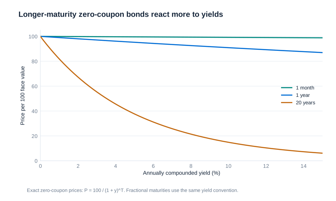
A single yield to maturity summarises the price of one instrument. It should not be mistaken for an assumption that every maturity in the market has the same discount rate. For more general fixed cash flows, valuation uses discount factors at each payment date; a yield to maturity is the single rate that reproduces the resulting total price under a chosen compounding convention.
Coupon bonds, par values and the term structure
A coupon bond distributes part of its value before the final redemption date. For annual coupons of amount , face value and an integer maturity , its single-yield pricing formula is
Each coupon and the principal must be discounted. When the coupon rate equals the required yield under the same payment convention, a conventional bond trades at par. A coupon rate below the required yield produces a price below par; a coupon rate above it produces a price above par. The discount or premium compensates the investor for the difference between contractual coupon income and the return required by the market.
| Annual coupon rate | Annual coupon | Calculated price | Price relative to par |
|---|---|---|---|
| 3% | 3 | 95.5482 | Below par |
| 4% | 4 | 100.0000 | At par |
| 5% | 5 | 104.4518 | Above par |
Under a nonflat term structure, the more general representation is , where is the cash flow at time and is the corresponding discount factor. A five-year annual-coupon bond can be treated as a portfolio of five zero-coupon claims: the first four pay coupons and the fifth pays coupon plus principal. This decomposition becomes important when different parts of the yield curve move by different amounts.
Macaulay duration as present-value-weighted timing
Macaulay duration measures the average time at which a bond's value is received, using present values as weights. Let be the present value of payment , let and define . Then
The weights sum to one for a positive-cash-flow bond, and duration is measured in years when payment times are measured in years. A ten-year zero-coupon bond has Macaulay duration ten years because all its value arrives at the final date. A coupon bond normally has a shorter Macaulay duration than its final maturity because some cash flows arrive earlier.
Portfolio duration is a market-value-weighted average under consistent conventions. Equal market-value investments in six-year and ten-year zero-coupon bonds give years of Macaulay duration. Equal face values would not generally give equal market-value weights. The distinction matters because risk sensitivity depends on today's economic values rather than simply the nominal amounts printed on the instruments.
The timing interpretation is particularly useful for relating assets to liabilities. Matching a portfolio's duration to the timing sensitivity of a future obligation can reduce first-order exposure to a small parallel rate change. It does not ensure that every cash flow occurs on the right date, eliminate reinvestment uncertainty under every rate path or provide protection against arbitrary changes in the curve's shape.
Modified duration and the value of a basis point
Modified duration converts cash-flow timing into first-order price sensitivity. For a nominal annual yield compounded times per year,
Here is the number of coupon or compounding periods per year, is expressed as a decimal annual rate, and is an absolute change in that rate. A rise from 4% to 5% is , not 1 and not a 25% relative yield change. The negative sign means that a positive-duration asset loses value when its yield rises.
One basis point, abbreviated bp, is 0.01 percentage points, or 0.0001 in decimal rate units. The positive magnitude of the approximate loss from a one-basis-point yield increase is often called PVBP, DV01 or the value of a basis point:
For the 20-year zero-coupon example at exactly 4.68%, and currency units per bp. A ten-basis-point rise therefore implies an approximate loss of 0.7654. Some systems report a signed PV01 sensitivity rather than a positive loss magnitude; the convention must be checked before combining positions or calculating hedge quantities.
Convexity and the limits of a linear approximation
Duration is the tangent slope of the price–yield relationship at the current yield. It becomes less accurate as the rate change grows because the slope itself changes. Price convexity, denoted , is the second derivative of price divided by price. A second-order approximation is
For a zero-coupon bond under annual compounding, . The 20-year example has convexity approximately 383.2850. For conventional positive fixed cash flows, convexity is positive: compared with the tangent approximation, the exact price is higher after either an upward or a downward yield shock. Duration alone therefore overstates the loss from a rise and understates the gain from a fall, for the same absolute shock.
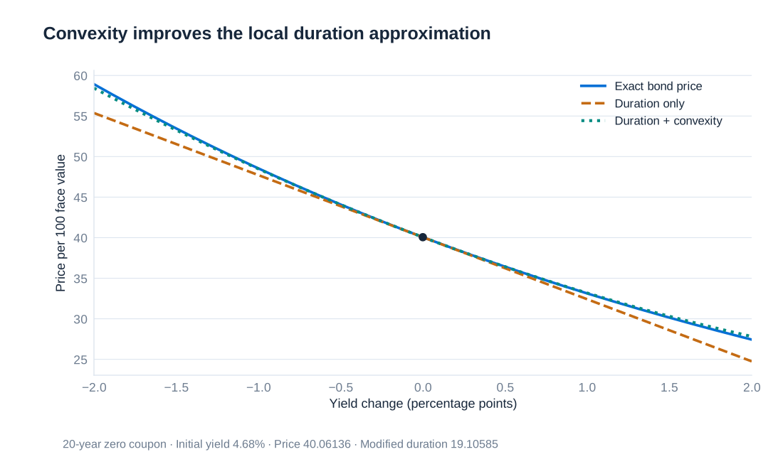
| Yield change | New yield | Exact repriced value | Duration approximation | Duration and convexity approximation |
|---|---|---|---|---|
| +0.01 | 5.68% | 33.124086 | 32.407300 | 33.175047 |
| −0.01 | 3.68% | 48.540051 | 47.715425 | 48.483171 |
The second-order calculation is considerably closer here but remains an approximation. Instruments with options can have different curvature because their expected cash flows change when rates change. Moreover, one duration and one convexity measure describe movement along one specified yield direction. They do not automatically capture twists, steepening or changes in credit spreads.
Hedging a bond portfolio with futures
Consider a corporate-bond portfolio worth USD 10 million with modified duration nine years. A one-basis-point parallel increase in its required yields produces an approximate value change of dollars. Suppose one long Treasury-bond futures contract loses approximately USD 90 for the corresponding one-basis-point increase. An offsetting hedge requires
The minus sign means 100 short futures contracts. If the matched rate movement occurs, the short futures gain approximately USD 9,000 while the bond portfolio loses approximately USD 9,000. This neutralises the specified first-order parallel-rate sensitivity. It does not make the entire portfolio risk-free or ensure zero profit and loss under all market changes.
Corporate-bond spreads can change relative to government yields; the portfolio and futures can have different convexity and maturity exposures; and the yield curve may move non-parallelly. The futures sensitivity can itself depend on delivery terms and the bond expected to be cheapest to deliver. Hedge ratios therefore require monitoring and rebalancing. Futures settlement also creates cash flows before bonds are sold, so sufficient liquidity is needed even when economic value changes offset.
Defining bond Value at Risk and the modelling horizon
Value at Risk, or VaR, is a selected quantile of a defined loss distribution over a defined horizon. If denotes a positive loss and is the confidence level, then . A 95% VaR is not a worst possible loss: the model assigns 5% of outcomes to losses exceeding that threshold. The cash flows, valuation date, holding period and treatment of carry must be stated.
Four simple methods can be illustrated with the same zero-coupon pricing function. One can model yield changes or directly model repriced bond changes, and one can use empirical quantiles or a normal-distribution approximation. These choices affect the result independently. A nonlinear pricing function can transform a symmetric yield distribution into an asymmetric price-change distribution.
| Method | Distribution assumption | Translation into loss |
|---|---|---|
| Historical yield quantile | Empirical distribution of yield changes | Adverse yield quantile multiplied by PVBP |
| Normal yield model | Normally distributed yield changes | Normal quantile, yield volatility and PVBP |
| Historical full repricing | Empirical yield scenarios applied to today's bond | Loss quantile from the repriced scenarios |
| Normal price-change model | Normal approximation to repriced price changes | Normal quantile multiplied by price-change volatility |
The numerical illustration uses weekly changes and therefore a one-week horizon. Mixing weekly volatility with a one-day VaR label changes the meaning of the result. The simple shock calculations below hold remaining maturity fixed while applying a yield change, isolating market-rate risk. A full one-week holding-period valuation should also reduce remaining maturity and include any cash flows or financing over the week; those adjustments must be applied consistently across all methods.
Historical yield shocks and the duration-based loss calculation
Suppose the empirical 95th percentile of weekly yield changes is an increase of 9.77 bp and the 5th percentile is −8.60 bp. For a long positive-duration bond, the upper yield tail is the adverse direction. Using the calculated PVBP gives
The equivalent duration calculation uses . The approximate fractional price loss is , or about 1.8666%. Multiplying by the price 40.061363 gives the same loss of approximately 0.748. Entering 0.00977 would mean a 97.7 bp shock and make the first-order loss ten times too large.
This estimate combines an empirical yield distribution with a linear value approximation. It is conditional on the selected historical period, data quality and quantile convention. A change in those inputs can change the result without any change in the bond itself. The relevant adverse tail would reverse for a short position, and a portfolio with options might not have a globally monotonic response to the same yield factor.
Normal yield shocks and full historical repricing
For a zero-mean normal model of weekly yield changes with standard deviation , the 95% first-order VaR is
With a weekly standard deviation of 5.443 bp, the result is currency units. The factor 1.645 is a one-sided 95% normal quantile; using 1.96 would instead correspond to a different tail probability. If a nonzero expected change is included, it must be carried through the loss model rather than silently omitted.
Historical full repricing avoids the duration approximation. For each observed or specified shock , calculate , then form the price change and loss . The following scenarios use yield changes expressed in bp; they are valuation calculations, not a claim that these few rows constitute the whole estimation sample.
| Yield shock, bp | Scenario yield | Scenario price | Price change |
|---|---|---|---|
| −5.0 | 4.630% | 40.4460 | +0.3846 |
| +2.3 | 4.703% | 39.8857 | −0.1756 |
| +5.1 | 4.731% | 39.6730 | −0.3884 |
| +4.0 | 4.720% | 39.7564 | −0.3049 |
| −3.1 | 4.649% | 40.2994 | +0.2380 |
| +13.1 | 4.811% | 39.0717 | −0.9896 |
| −1.0 | 4.670% | 40.1380 | +0.0766 |
| −6.2 | 4.618% | 40.5389 | +0.4775 |
| −3.7 | 4.643% | 40.3456 | +0.2843 |
| −1.8 | 4.662% | 40.1994 | +0.1380 |
| +1.7 | 4.697% | 39.9315 | −0.1299 |
| −2.9 | 4.651% | 40.2840 | +0.2226 |
| +8.5 | 4.765% | 39.4163 | −0.6451 |
| +6.2 | 4.742% | 39.5897 | −0.4716 |
| −8.2 | 4.598% | 40.6942 | +0.6328 |
| −11.8 | 4.562% | 40.9753 | +0.9140 |
| −1.7 | 4.663% | 40.1917 | +0.1303 |
| +4.8 | 4.728% | 39.6957 | −0.3656 |
| −13.5 | 4.545% | 41.1088 | +1.0474 |
| +5.8 | 4.738% | 39.6200 | −0.4414 |
For the same adverse 9.77 bp shock used in the linear model, full repricing gives . Positive convexity explains why this loss is slightly smaller than 0.747802. With a monotonic fixed-maturity price function, a consistently defined empirical upper yield quantile maps to the corresponding upper loss quantile, subject to the interpolation convention. One should not interpret a materially different value as a convexity effect without checking that the samples and signs match.
A normal model for price changes and numerical consistency
The fourth method estimates the standard deviation of repriced bond changes and then imposes a normal approximation directly on those changes. If their standard deviation is 0.417 currency units and their mean is neglected, the 95% VaR is . Yield-normal and price-normal models can give similar numbers for small shocks, but they are different assumptions because the bond price is a nonlinear function of yield.
An illustrative comparison based on weekly 2024 observations reports rounded VaR figures of 0.75 from the empirical yield quantile, 0.68 from the normal yield model, 0.66 from an empirical price-loss quantile and 0.69 from the normal price-change model. Its price-change summaries are a 5th percentile of −0.66, a 95th percentile of +0.72 and a standard deviation of 0.417. These are separate reported summary statistics, not enough information to reconstruct a complete common sample. In particular, the 0.66 empirical loss cannot be reproduced by applying the stated 9.77 bp adverse quantile to this fixed-maturity bond; the consistent calculation gives approximately 0.741.
The useful lesson is the method comparison, together with the requirement to reconcile inputs. A 95% loss quantile is the negative of the 5% price-change quantile, not the positive 95% price-change quantile. Small changes around 0.685 can also round to either 0.68 or 0.69 when underlying inputs have already been rounded. A robust calculation keeps unrounded prices and sensitivities, aligns observation frequency and sample dates, and applies a common loss convention before comparing model outputs.
Multiple yield-curve factors and instrument optionality
A coupon bond does not have only one economically relevant interest rate. Its component payments depend on discount factors at different maturities. Historical simulation can apply a joint observed change in the one-, two-, three-, four- and five-year rates to a five-year bond, then revalue all payments. The rate changes must come from the same historical observation so that their dependence is preserved.
For a first-order parametric model, let be a vector of decimal changes in the chosen curve rates, let contain the corresponding currency sensitivities , and let be the covariance matrix of those changes. Then
Adding separate maturity risks without covariance terms would miss the way curve movements reinforce or offset one another. Key-rate sensitivities make this structure visible. Similar valuation and scenario methods apply to interest-rate swaps and futures, with contract-specific cash flows and settlement conventions. Callable bonds, convertible bonds and bond options require additional modelling because exercise decisions or other risk factors can change the cash flows themselves.
Risk horizons, pull to par and a shrinking duration
A default-free zero-coupon bond pays its face value at maturity regardless of the path of interim market yields. As maturity approaches, its remaining duration falls and its price converges to that payment. Conditional on a similar distribution of yield shocks, its near-term interest-rate price sensitivity therefore decreases. This is a changing exposure, not a reason to apply the same volatility estimate mechanically at every future date.
If the horizon is exactly the maturity date, the nominal redemption cash flow is certain under the default-free assumption. The dispersion of that terminal payment due solely to interest-rate uncertainty is zero. It does not follow that every definition of investment loss or every investor's risk is zero: the comparison benchmark, purchase price, inflation and liquidity needs still matter. A coupon bond additionally creates reinvestment uncertainty for payments received before the horizon.
A short-term trader may need to know tomorrow's liquidation loss, whereas a saver concerned with retirement wealth in 2065 needs a model of cash flows and reinvestment over a much longer period. The horizon should follow the economic decision. Extending a short-horizon VaR by a square-root rule without considering declining maturity, changing sensitivities and cash flows can produce misleading results for bonds held over long periods.
Economic value of equity and the banking-book duration gap
Interest rate risk in the banking book, abbreviated IRRBB, concerns the effect of interest-rate movements on a bank's economic value and earnings outside its trading activities. Let and be the present values of assets and liabilities, and let be economic equity. If and are their modified durations under a common small parallel yield shock, then
The liability term must be subtracted because equity equals assets minus liabilities. A decline in the economic value of a liability benefits equity, other things equal, whereas a decline in asset value reduces it. Writing gives the equivalent expression .
For an illustrative bank with assets of 100, liabilities of 90 and equity of 10, take asset duration five years and liability duration zero. A parallel rise of 200 bp, or 0.02, gives , equal to the initial equity in magnitude. This is a first-order economic-value stress, not a statement that an accounting loss of exactly 10 must immediately be booked. If liability duration were two years instead, the approximate change would be .
Basel's IRRBB framework considers both economic-value and earnings measures and includes parallel and non-parallel interest-rate scenarios. A single 200 bp shock is useful for exposition and historical comparison, but it is not a complete modern stress framework. Steepening, flattening and movements concentrated at short maturities can reveal exposures concealed by a small aggregate duration gap.
Regulatory reference: Basel Framework SRP98, guidance on interest-rate risk in the banking book.
Deposit behaviour and historical evidence from German banks
The effective sensitivity of retail deposits is difficult to infer from legal maturity alone. A sight deposit can be withdrawn immediately, but a stable portion of aggregate balances may remain with the bank for years. At the same time, the rate paid to depositors may adjust slowly or rapidly when market rates change. Balance stability, contractual withdrawal rights and the repricing of deposit rates are related but distinct modelling questions. An average historical holding period is not automatically the correct duration.
Assuming a long behavioural duration for deposits can reduce the estimated duration gap against long fixed-rate assets. If customers withdraw funds, demand higher rates or move from sight deposits to time deposits during stress, that assumed protection can weaken. Behavioural assumptions must therefore be tested across scenarios and linked to the bank's funding strategy rather than accepted merely because past balances appeared stable.
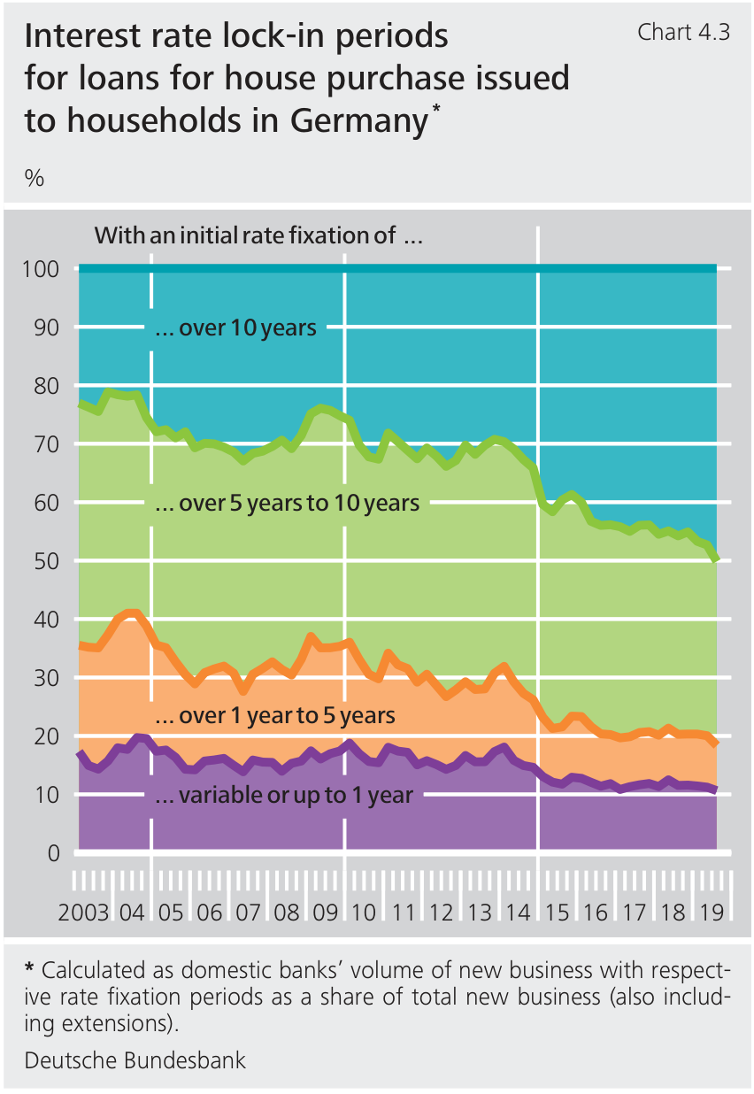
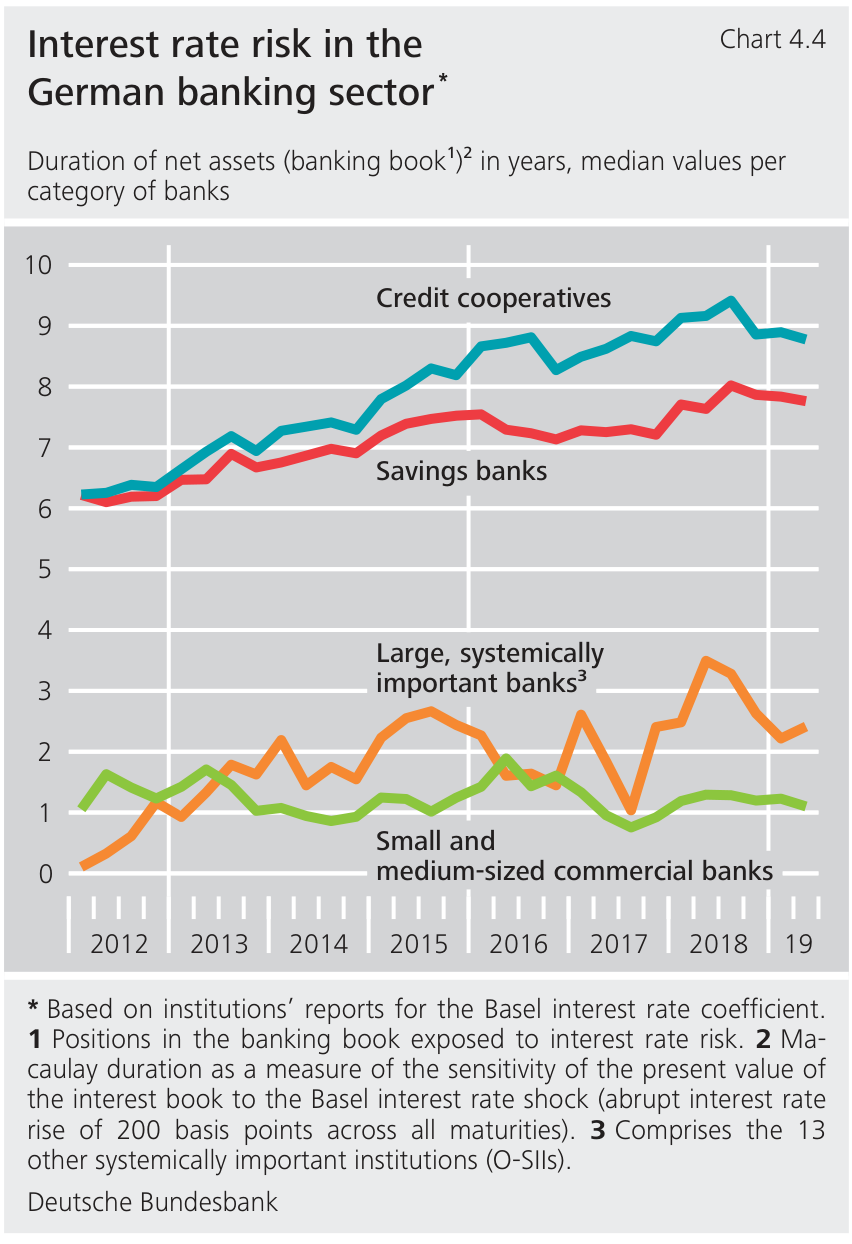
The historical German mortgage evidence shows a growing share of new household house-purchase lending with initial rate fixation longer than ten years during 2003–2019. The accompanying banking-sector measures show that duration exposure differed substantially across credit cooperatives, savings banks and commercial-bank groups. The composition of new loans is not identical to the duration of the whole existing balance sheet, but it helps explain how prolonged low-rate conditions could increase fixed-rate asset exposure.
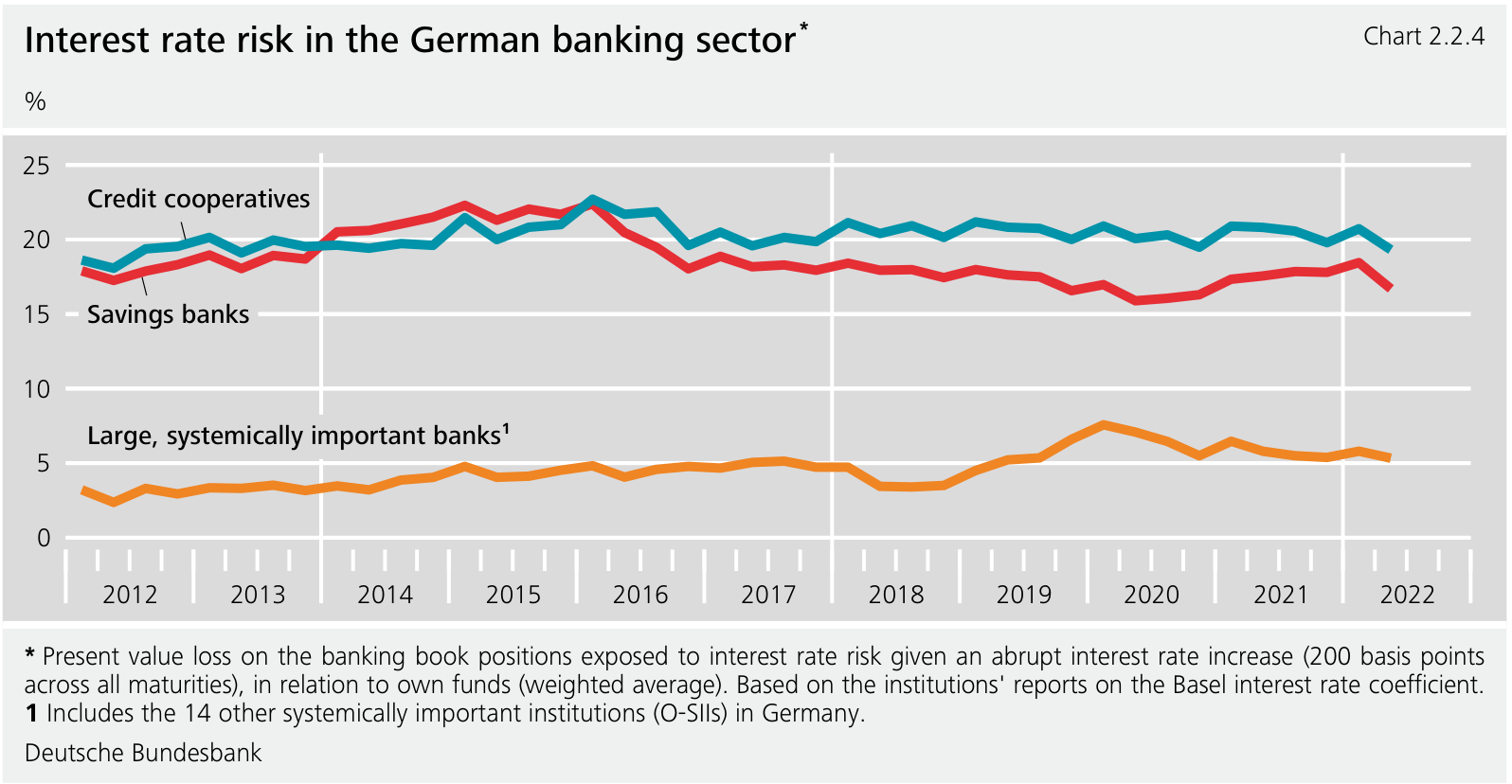
The Bundesbank's 2022 historical comparison expresses the present-value loss from a 200 bp upward shock as a percentage of own funds. Savings banks and credit cooperatives had larger reported ratios than the group of large systemically important banks in that series. These are category-level measures with specified weighting and reporting conventions, not the same as the loss rate on assets or a conclusion about every institution in each group.
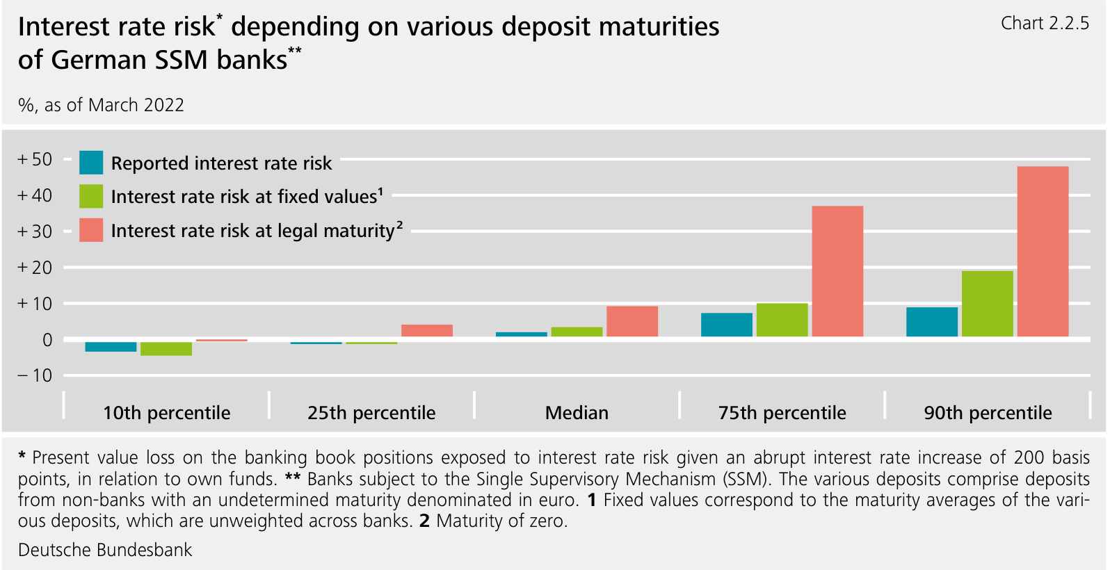
A separate March 2022 comparison for German banks under the Single Supervisory Mechanism contrasts reported deposit assumptions with fixed average maturities and legal maturity of zero for relevant nonbank euro deposits. The upper percentiles of measured risk rise substantially under the legal-maturity treatment. The comparison demonstrates model sensitivity: the economic-value estimate depends not only on observed market prices but also on assumptions about how deposit balances behave.
Repricing gaps and net interest income
Economic value is a present-value measure over future cash flows; net interest income, or NII, is interest revenue minus interest expense over a period. A bank can experience a fall in the market value of long fixed-rate assets while its current interest margin initially improves because some asset rates reset faster than deposit costs. Conversely, funding costs can increase before fixed asset income adjusts. The value and earnings perspectives are complementary, not interchangeable.
In a simplified one-period repricing model, let denote assets whose rates reset within the horizon and the corresponding liabilities. If both reprice immediately and fully to the same rate change, the approximate annualised income effect is
For hypothetical rate-sensitive assets of EUR 60 million and liabilities of EUR 80 million, the gap is EUR −20 million. A two-percentage-point increase implies an annualised NII change of million euros. Actual within-year effects depend on reset dates, rate pass-through, floors and business volumes. This gap is measured in currency and differs from the duration gap used to approximate economic-value changes.
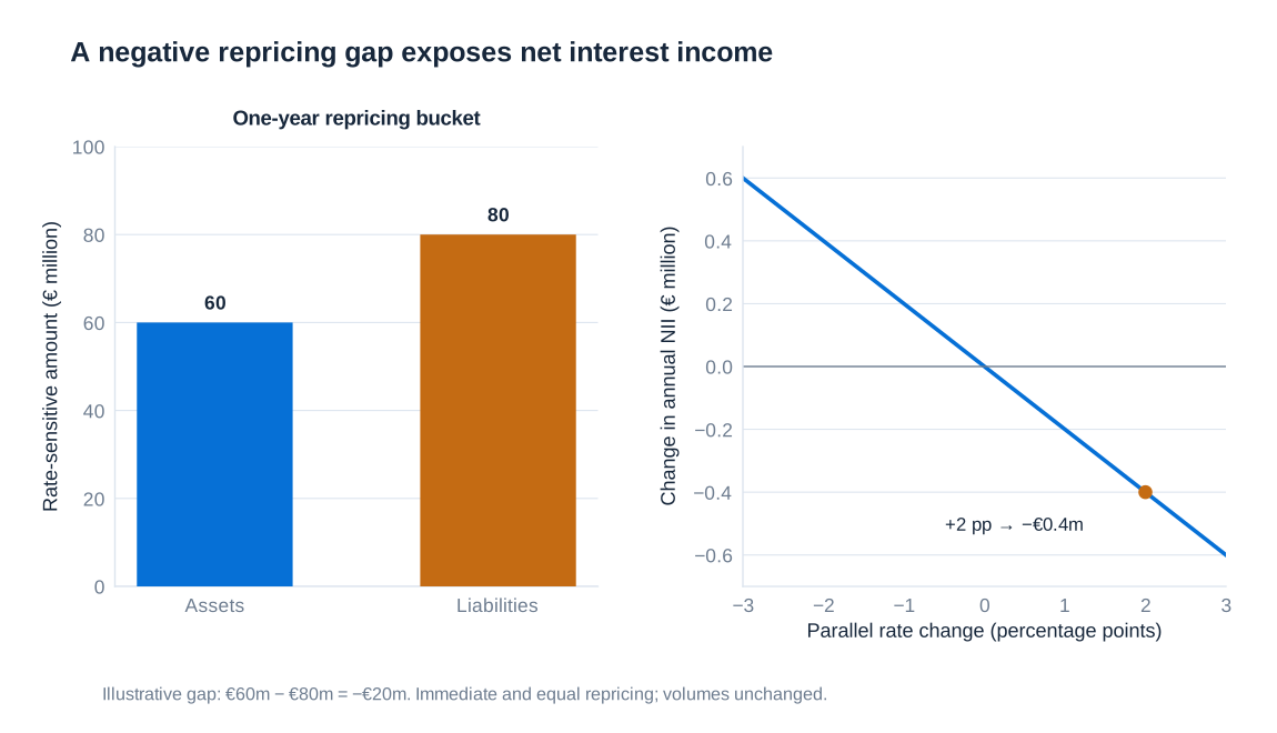
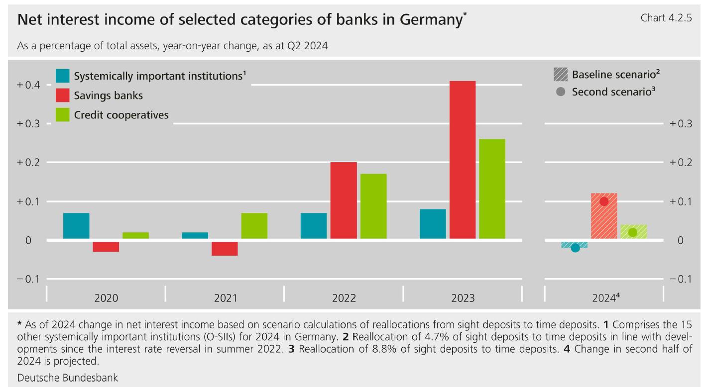
The Bundesbank's comparison through the second quarter of 2024 distinguishes realised annual changes in net interest income from scenario calculations for 2024. It shows stronger improvements for savings banks and credit cooperatives after the interest-rate reversal, while the projected effect depends on customers moving funds from sight deposits into more highly remunerated time deposits. Scenario bars should not be read as subsequently realised outcomes.
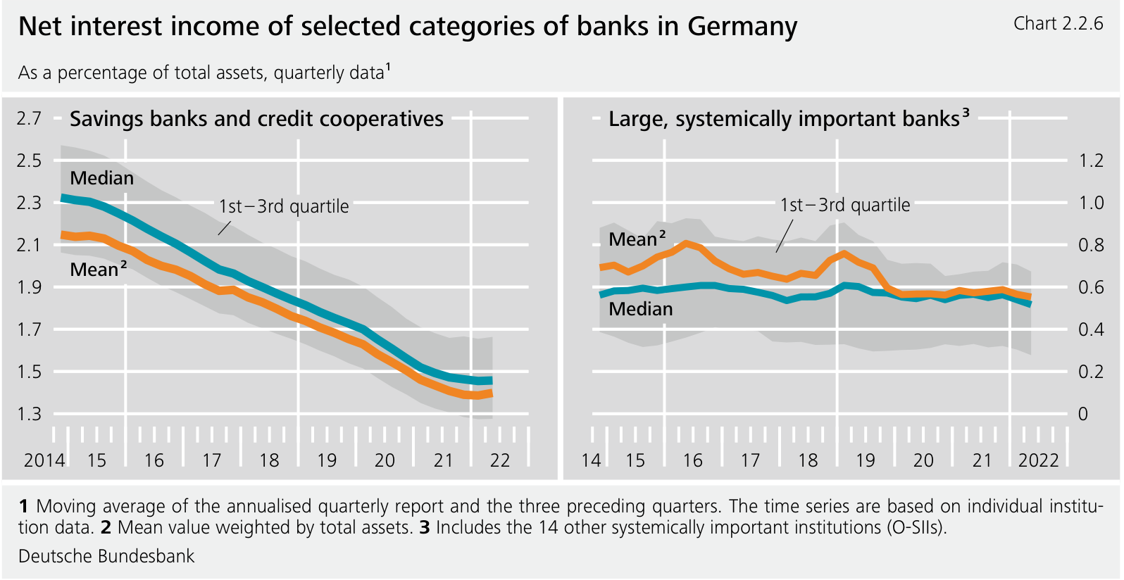
The longer 2014–2022 series shows declining NII relative to total assets for savings banks and credit cooperatives during much of the low-rate period. Large systemically important banks are shown on a separate scale and have different business mixes. The median, asset-weighted mean and interquartile range summarise different features of the distribution; comparing line heights without checking axes or weighting can give a misleading conclusion.
Amortised cost, hidden reserves and unrealised losses
Accounting carrying amounts and market values answer different questions. An instrument carried at amortised cost does not generally have its carrying amount reset to current fair value after every market-rate movement. Its economic value can nevertheless change materially. A market value above the relevant carrying value creates an unrealised gain, often described as a hidden reserve in this context; a market value below it creates an unrealised loss. Hidden reserves are not another name for losses.
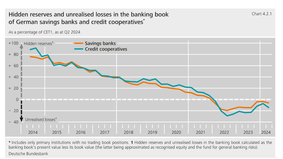
The historical Bundesbank series for German savings banks and credit cooperatives, expressed relative to Common Equity Tier 1 capital and extending to the second quarter of 2024, shows earlier positive differences turning negative around the 2022 rate increase. Its definition compares the banking book's present value with its book-value approximation. The chart illustrates a valuation gap under that stated methodology, not an automatic deduction of the whole amount from reported regulatory capital.
If a bank can hold assets and finance them as planned, an unrealised market loss need not require immediate liquidation. If deposits leave or collateral needs rise, sales can crystallise losses and reveal the connection between interest-rate risk and funding liquidity. Effective management therefore combines economic-value stress tests, earnings projections, behavioural deposit analysis and cash-flow capacity. The label “banking book” or “amortised cost” does not remove the underlying economic sensitivity.
5. Option-Related Risks and Greeks
Market value, terminal payoff and profit
An option creates a contingent right rather than an unconditional obligation for its buyer. A call gives its holder the right to buy the underlying at the strike price; a put gives the right to sell. The writer receives the premium and accepts the corresponding obligation. Let denote the underlying price at time , the strike, the expiry date, and or the market value of a call or put. All prices and premiums in a particular example are expressed in the same currency per unit of underlying. Contract multipliers convert these unit amounts into the cash exposure of actual contracts.
The terminal payoff is the contractual amount received at expiry. Profit also accounts for the premium and, in a complete investment calculation, financing, transaction costs and any other cash flows. Unless stated otherwise, the terminal-profit examples below subtract the initial premium without accumulating interest. This convention makes the payoff geometry transparent; it is not a claim that financing is free in actual trading.
A call with strike EUR 25 purchased for EUR 2.50 can lose market value before expiry even while the underlying remains above EUR 25. Its resale price depends on the underlying, remaining time, implied volatility and interest rates. If the call expires with , its payoff is zero and the buyer loses the EUR 2.50 premium. If , it pays EUR 1 but the buyer still has a net loss of EUR 1.50. Ignoring financing, break-even is EUR 27.50. An option finishing in the money is therefore not necessarily a profitable investment.
Intrinsic value is the immediate-exercise value, for a call and for a put. The difference between market value and intrinsic value is conventionally called time value. For options with an immediate-exercise right it is non-negative under usual no-arbitrage conditions; for European options, discounting and exercise restrictions mean that comparison with immediate intrinsic value requires care. A positive remaining maturity should never be treated as guaranteeing a particular time-value sign for every contract.
| Position | Profit per unit | Maximum loss | Maximum profit |
|---|---|---|---|
| Long call | Unbounded if the underlying price has no upper bound | ||
| Short call | Unbounded if the underlying price has no upper bound | ||
| Long put | when | ||
| Short put | when |
Here and are premiums paid by buyers and received by writers; the put bounds assume a non-negative underlying price. For an underlying that can become negative, those bounds must be reconsidered. “Naked” describes an option position without the relevant offsetting exposure. A short call backed by shares has a different aggregate risk profile from a naked short call, even though the option leg itself is identical.
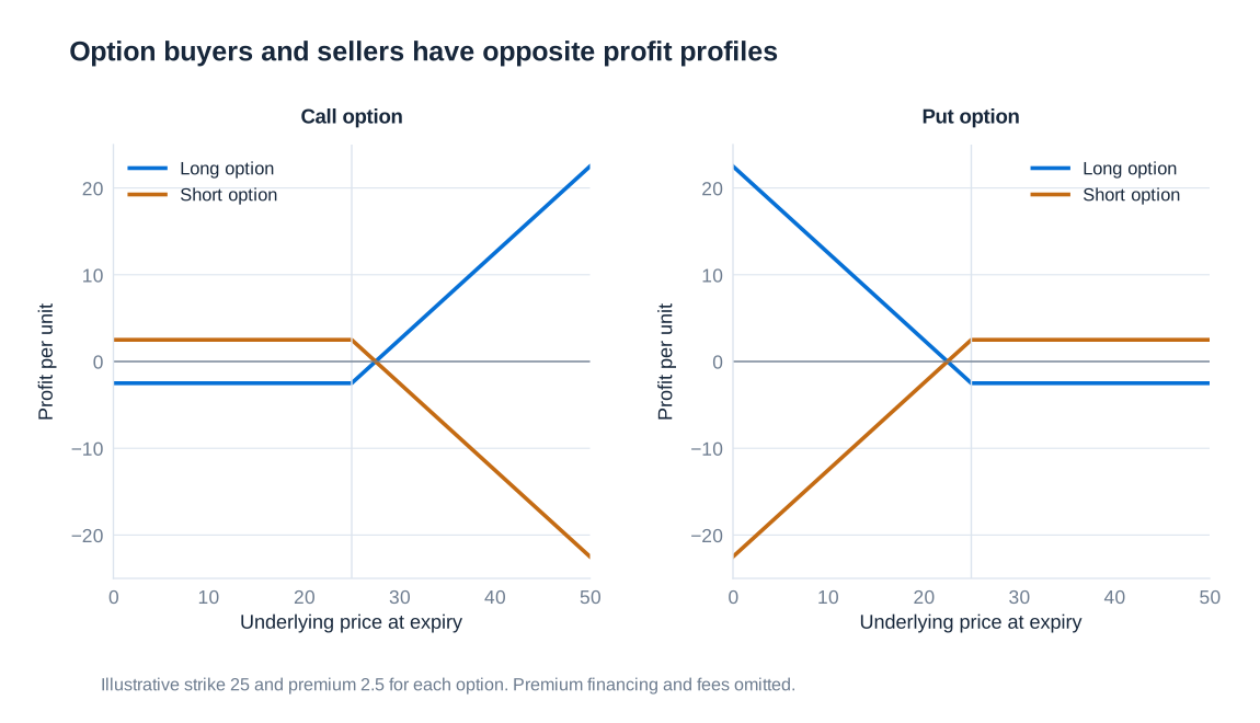
A bull call spread: constructing a bounded position
A bull call spread expresses a moderately positive view while limiting both the premium at risk and the benefit from a large price increase. Buy a call with lower strike and sell a call with higher strike , using the same underlying, expiry and unit quantity. If the premiums are and , the net premium paid is . The terminal profit is:
Consider a stock initially trading at USD 50. A strike-50 call costs USD 3, and a strike-55 call can be sold for USD 1. The initial debit is USD 2. Below the lower strike both calls expire worthless; between the strikes only the purchased call pays; above the higher strike the two exercise values rise at exactly the same rate, so their difference stops increasing.
| Terminal stock price | Long-call payoff | Short-call payoff | Net profit |
|---|---|---|---|
| USD 45 | USD 0 | USD 0 | −USD 2 |
| USD 50 | USD 0 | USD 0 | −USD 2 |
| USD 52 | USD 2 | USD 0 | USD 0 |
| USD 53 | USD 3 | USD 0 | USD 1 |
| USD 55 | USD 5 | USD 0 | USD 3 |
| USD 60 | USD 10 | −USD 5 | USD 3 |
The maximum loss is USD 2, the maximum profit is dollars, and break-even is dollars. The maximum payoff is USD 5, which differs from the maximum profit. These amounts are per unit: a spread using contracts covering 100 shares has a USD 200 initial debit and USD 300 maximum terminal profit, before fees and financing.
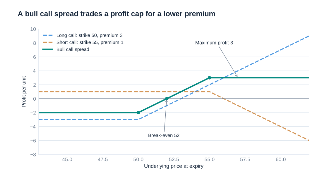
The terminal bound does not describe every operational exposure. If an American-style short call is assigned early, the investor may acquire a stock delivery obligation before the long call is exercised or sold. Funding, dividends and transaction costs can then affect realised results. The economic spread should be analysed together, while exercise and settlement obligations must also be managed leg by leg.
Equivalent shapes and the bull put spread
A bull put spread buys the lower-strike put and sells the higher-strike put. Its terminal option payoff is . This is the bull call spread’s payoff minus the constant . Consequently, the two option packages do not have identical raw cash payoffs. Their risk-dependent shapes are the same, with the difference accounted for by a fixed payment and the corresponding financing.
For European options with common maturity, put–call parity links their initial prices. With a constant continuously compounded rate , the call-spread debit equals the put-spread debit plus , taking the valuation date as zero. A matching risk-free cash position therefore converts one strategy into the other. Comparing only the names “calls” and “puts” conceals this equivalence; comparing only terminal profits without a financing convention can also conceal a genuine cash-flow difference.
At zero interest, the strike-50/55 call spread costing 2 corresponds to a bull put spread receiving a credit of 3. Below 50 the put spread pays −5, giving profit −2 after its initial credit; above 55 it pays zero and retains profit 3. The same break-even and maximum profit or loss follow. The example demonstrates why portfolio risk analysis must aggregate contractual cash flows and premiums before deciding whether a position is bullish, bearish or bounded.
Straddles, butterflies and the price of convexity
A long straddle purchases a call and a put with the same strike and expiry. Its terminal payoff is , and its profit is . The buyer benefits from a sufficiently large move in either direction, not merely from any movement. With total premium , break-even prices are and , provided the lower one is feasible for the underlying. The maximum loss is the premium, occurring when the terminal price equals the strike.
As an explicitly illustrative example, take and total premium 12. The break-even prices are 38 and 62. Expiry at 40 still produces a loss of 2 because the payoff of 10 does not recover the premium. Expiry at 70 produces profit 8. Before expiry, the value can increase when implied volatility rises even if the underlying price barely moves; an eventual terminal profit also depends on how much movement was already priced into the options.
A short straddle reverses these profits. The writer retains the total premium when the underlying finishes at the strike, but faces losses for sufficiently large moves. For a non-negative equity price the downside-price loss is bounded by , while the upside-price loss is unbounded. A calm historical sample can make this strategy appear attractive even though a rare large move creates severe losses. Margin calls can force liquidation before the terminal payoff is reached.
A long call butterfly buys one call at , sells two at , and buys one at , with equally spaced strikes and common expiry. Its payoff is:
The payoff is zero outside the two outer strikes and reaches at the middle strike. Subtract the net debit to obtain profit. With illustrative strikes 45, 50 and 55 and debit 2, the maximum loss is 2, maximum profit 3 and break-even prices 47 and 53. The purchased wings limit tail losses relative to an unprotected short-volatility position. Adding appropriate wings to a short straddle produces an iron-butterfly structure; a call butterfly is a related bounded structure, not literally a long straddle with two arbitrary extra options.
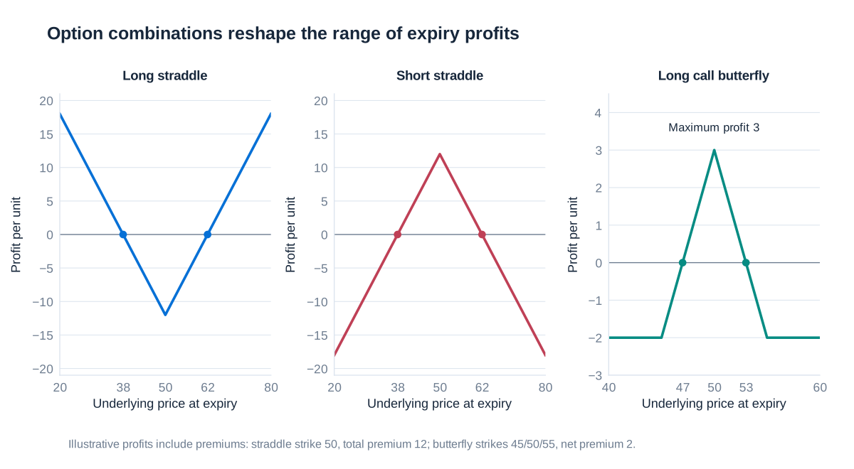
The Greeks as local sensitivities
Terminal diagrams hold the expiry date fixed and vary the final underlying price. Daily risk management asks a different question: how much will the current option value change when market inputs move? Write , where is annualised implied volatility, the relevant rate, and calendar time. A local Taylor expansion separates major sources of profit and loss:
| Greek | Definition | Interpretation |
|---|---|---|
| Delta | First-order value change per unit change in the underlying price | |
| Gamma | Change in delta per unit underlying-price change; determines local curvature | |
| Vega | Value sensitivity to implied volatility in the chosen volatility units | |
| Rho | Value sensitivity to the chosen interest-rate input | |
| Theta | Value change from calendar time passing, with other inputs held fixed |
The symbol is used both for a Greek and, when preceding a variable, for a change; the product means option delta multiplied by the price change. If instead time to maturity is the pricing input, calendar-time theta is . Confusing these conventions reverses the reported sign. A theta calculated per year must also be converted consistently before applying a one-day change.
Volatility of 20% is 0.20 in decimal form. An increase to 21% is one percentage point, meaning , not 1. A raw vega derivative of EUR 500 per unit decimal volatility implies approximately EUR 5 for that change. Trading systems often report vega directly per percentage point and rho per basis point or percentage point. Units must therefore accompany each number. FX options may require sensitivities to both domestic and foreign interest rates. If is the foreign rate, the expansion adds with . Complex portfolios need term-structure and volatility-surface buckets rather than one universal rate or volatility.
The expansion omits higher powers and cross-derivatives, including interactions between price and volatility. Its accuracy deteriorates for large shocks, near discontinuities and when important inputs are missing. Gamma improves on delta alone, but delta–gamma is still an approximation. Full revaluation under joint scenarios is the appropriate comparison when assessing whether the local approximation remains useful.
Aggregating Greeks into a usable risk report
Portfolio Greeks add across positions when they refer to the same risk factor, units and valuation conventions. For signed quantities and contract multipliers , portfolio delta is , and analogous expressions apply to the other Greeks. Long and short positions can offset in one sensitivity while reinforcing another. A near-zero aggregate delta is compatible with substantial gamma or vega exposure.
Consider an explicitly illustrative portfolio worth EUR 150 million with 120 positions in equities, indices and commodities. To make an aggregate scenario report interpretable, define a common parallel relative-price shock , a volatility shock , a rate shock , and elapsed time in days. These are standardised scenario coordinates, not claims that different underlyings always move together. The following local coefficients are in EUR millions:
| Sensitivity | Reported value | Meaning in the scenario approximation |
|---|---|---|
| Price delta | 10 | EUR 10 million first-order gain for a 1% parallel price increase |
| Price gamma | 2 | Second derivative with respect to ; contributes million |
| Vega | 5 | EUR 5 million gain per one-percentage-point volatility increase |
| Theta | −1 | EUR 1 million loss per day from time passing |
| Rho | 3 | EUR 3 million gain per one-percentage-point rate increase |
A 5% parallel price decline has : the delta contribution is −50 million and the gamma contribution is +25 million, giving a local delta–gamma estimate of −25 million. Reporting only −50 million is a first-order calculation, not a calculation that incorporates the stated gamma. A ten-percentage-point volatility increase gives a vega-only gain of 50 million, whereas a 10% relative increase from 20% to 22% volatility gives only 10 million. A half-percentage-point rate increase gives 1.5 million. These isolated calculations hold other inputs fixed; large joint stresses require full revaluation.
A practical report also separates underlyings, maturities and volatility buckets, identifies large concentrations, and shows the effect of proposed hedges. The number of positions and market value help describe scale but do not measure risk by themselves. Reporting a Greek simply as a currency amount without specifying its shock normalisation can produce errors larger than the apparent precision of the calculation.
Delta hedging and the residual gamma exposure
Suppose a purchased call has delta 0.6 and covers one share. A USD 1 increase in the share price gives an approximately USD 0.60 call gain. Shorting 0.6 shares creates an approximately USD 0.60 loss on the stock leg, cancelling the first-order effect. The hedge reverses for a short call: the writer buys shares. This is a local hedge at the current price, not a statement that all possible price movements now have zero consequences.
A trader short 100 calls on SAP, each covering one share and each with delta 0.6, has option delta −60. Holding 60 SAP shares makes combined delta zero. If each actual contract covers 100 shares instead, the required stock position is 6,000 shares. Contract-count and underlying-unit conventions must be reconciled before a hedge is executed.
Shares have zero gamma, so they cannot remove the option position’s curvature. A short conventional call has negative gamma. In an explicitly illustrative local example, a long call’s value around is approximated by . The short-100-call portfolio plus 60 shares then has price-driven change:
A move of either +1 or −1 produces an approximate loss of 2 currency units; a move of either +5 or −5 produces an approximate loss of 50. The quadratic expression is a local approximation rather than a globally valid option price. It isolates gamma while ignoring theta, financing and volatility changes. A long option with an offsetting short stock position has the opposite local curvature.
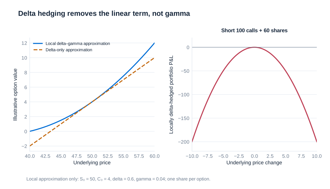
After a rise in the underlying, a call’s delta may increase from 0.6 to 0.9. The short-100-call hedger must then raise the stock holding from 60 to 90 shares. After a decline, the hedger generally sells shares as delta falls. This buy-after-rises and sell-after-falls pattern explains the rebalancing burden of short gamma. Transaction costs, market jumps, discrete hedge intervals and illiquidity prevent a dynamic hedge from being an unconditional guarantee. Delta hedging also leaves volatility, rate, basis and model risks unless these are separately managed.
Fuel options: economic protection and cash expenditure
An airline purchasing fuel is exposed to rising fuel prices. Buying calls can cap the price paid while preserving the benefit of falling prices, at the cost of an upfront premium. Consider a simplified quarterly requirement of 100 barrels, hedged by calls on exactly 100 barrels with strike USD 25 and premium USD 1.20 per barrel. Assume the options settle when the fuel is purchased, the underlying exactly matches the fuel price and there are no financing or transaction costs.
| Fuel price per barrel | Physical purchase cost | Option receipt | Premium | Net expenditure |
|---|---|---|---|---|
| USD 20 | USD 2,000 | USD 0 | USD 120 | USD 2,120 |
| USD 25 | USD 2,500 | USD 0 | USD 120 | USD 2,620 |
| USD 40 | USD 4,000 | USD 1,500 | USD 120 | USD 2,620 |
Above the strike, the option receipt offsets every additional dollar paid for the matched fuel quantity. Below the strike the option expires, but physical fuel becomes cheaper. Calling the expired option a failed hedge ignores the combined position. The premium buys protection; it is not expected to be recovered in every state of the world.
Net cash expenditure is not automatically the same as an accounting-period expense. Fuel may first enter inventory, premiums may be paid earlier, and hedge accounting may defer or reclassify components. Nor does this simple example capture real jet-fuel basis risk when the hedge references crude oil, mismatched delivery dates or uncertain fuel volumes. An airline must evaluate the matched economic exposure and the residual mismatches separately.
Time value and reported earnings: the Lufthansa example
A purchased fuel call can gain intrinsic value as fuel prices rise while losing time value as expiry approaches or implied volatility falls. The total derivative value is the sum of these components, but accounting rules may recognise their changes in different places or periods. Under a historical IAS 39 cash-flow-hedge designation that separated intrinsic value from time value, the effective designated component could be deferred in other comprehensive income, or OCI, while excluded time-value changes entered profit or loss. OCI is part of comprehensive income and equity; it is not the same as current-period net profit.
For an illustrative accounting bridge, suppose the intrinsic-value component increases by EUR 575 million while time value decreases by EUR 289 million. The derivative’s net value rises by EUR 286 million, yet a qualifying intrinsic-value-only designation could show the 575 million effective gain in OCI and the 289 million time-value loss in profit or loss, before tax and other adjustments. These illustrative amounts describe the mechanism; they should not be confused with cash settlements, total airline profit or a verified quarterly financial statement.
Lufthansa’s 2011 annual report provides a documented historical example: it reported EUR 96 million of adverse changes in option time value in the financial result, primarily from fuel hedges, while realised fuel-hedging gains reduced fuel costs by EUR 694 million. These are full-year figures. The accompanying accounting policy distinguished changes in intrinsic value recognised in equity from changes in time value recognised in the financial result. The economic assessment therefore required both the fuel bill and the hedging components, not an isolated derivative expense.
The historical treatment should not be applied mechanically to current accounts. IFRS 9 provides cost-of-hedging treatment for qualifying excluded option time value, with recognition depending on the hedge and whether it relates to a transaction or a period. Lufthansa’s first-quarter 2018 report describes a change to the recognition of option time values on adoption of IFRS 9. Entities may also elect to retain IAS 39 hedge-accounting requirements under the applicable IFRS 9 policy choice. Designation, effectiveness, documentation and the specific hedged item therefore remain essential.
The risk-management lesson is to distinguish economic cash-flow protection, derivative fair-value changes and reported earnings. A hedge can meet its economic objective while creating accounting volatility; conversely, a smooth reported earnings series does not prove that all economic exposures are hedged. Risk reports should explain the reconciliation and the periods in which hedging gains, fuel costs and option premiums affect the accounts.
Accounting and case references: Lufthansa Annual Report 2011; Lufthansa Interim Report, first quarter 2018; IFRS 9 overview; IFRS 9, paragraph 6.5.15.
6. Value at Risk Models and Market-Risk Measurement
What a market-risk measure is intended to describe
Market risk arises when portfolio value changes with interest rates, credit spreads, equity prices, exchange rates, commodity prices or implied volatilities. Banks, hedge funds, investment funds, pension funds, insurers, sovereign wealth funds, central banks and corporate treasuries all face versions of this problem. Their portfolios and objectives differ, but each needs to connect movements in market factors to losses that matter for its decisions. A corporate treasury may focus on foreign-currency assets or fuel hedges; a trading desk may focus on daily valuation changes; a pension fund must also consider liabilities and a longer horizon.
Different measures answer different questions. An exposure amount, such as EUR 2.5 million invested in dollar assets, describes scale but not the likelihood or severity of a euro loss. A sensitivity, such as delta, duration or the value of a basis point, describes a local response to one specified shock. Scenario analysis examines the consequences of a particular combination of shocks. Portfolio variance summarises dispersion around the mean. Value at Risk, or VaR, describes a quantile of a loss distribution; Expected Shortfall, or ES, describes the average severity of the specified tail. These measures complement rather than replace one another.
Accounting classification does not remove economic market risk. Trading positions are commonly measured at fair value through profit or loss, so price changes can affect reported earnings immediately. Banking-book assets and liabilities may be measured at amortised cost or under other accounting categories, while their economic values remain sensitive to rates and spreads. Analysis of interest-rate risk in the banking book consequently includes both economic-value and earnings perspectives. It is inaccurate to identify the entire trading book with one accounting rule or the entire banking book with amortised cost.
VaR as a loss quantile, not a maximum possible loss
Fix a valuation date, portfolio, reporting currency and risk horizon . Let be profit or loss over that horizon and define positive loss as . With an unchanged portfolio and explicit cash flows, one possible definition is , where contains relevant receipts net of payments. A static instantaneous-shock calculation may deliberately exclude future cash flows and time passage, but that is a modelling convention, not a universal property of VaR.
A one-day 99% VaR of EUR 10 million means that the model assigns at least 99% probability to a loss no greater than EUR 10 million. For a continuous distribution, the exceedance probability is 1%; with discrete outcomes it need not be exactly 1%. The measure says nothing by itself about whether an exceedance is EUR 10.1 million or EUR 100 million. Calling it the “maximum expected loss” confuses a quantile with both a worst-case bound and an expectation.
The confidence level is the chosen probability threshold for the modelled distribution. It is not a statistical confidence interval for the accuracy of the VaR estimate. A model can report 99% VaR while its parameter estimates remain highly uncertain. Nor does 99% imply only one loss event in a career: under correct independent daily modelling, about 2.5 exceedances would be expected in 250 trading days. Their occurrence is not automatically evidence that the model failed; their frequency, clustering and severity must be examined.
Ordinary VaR may use a recent historical calibration or a conditional forecast of current market conditions. Stressed VaR instead uses a stressed period or distribution appropriate to the portfolio’s exposures. Both remain quantiles. A stressed estimate need not be larger for every conceivable portfolio if the selected stress episode affects different risk factors; the choice must be justified by the actual positions. Reporting VaR without its horizon, confidence level, loss definition and calibration period makes meaningful comparison impossible.
From positions and market data to a portfolio loss distribution
A VaR system combines two streams of information. The position stream identifies contracts, quantities, contractual terms, currencies and valuation models. Mapping translates these holdings into exposures to relevant market factors. The market-data stream supplies observed prices, yield curves, spreads and volatility surfaces, from which a joint distribution of shocks is estimated or selected. Revaluing the same current portfolio under those shocks produces a distribution of hypothetical profit and loss. Quantiles and tail averages are calculated only after this aggregation.
This architecture explains why “add up each instrument’s VaR” is generally wrong. The portfolio distribution depends on which gains and losses occur together. Offsetting exposures can reduce risk, while positions with different labels can share the same underlying factor. A single bond may require several interest-rate curve points, a credit spread and a currency factor. An option additionally requires volatility and nonlinear valuation. Poor mapping can omit material risks even when the quantile calculation is numerically perfect.
Market observations must be aligned in time and expressed in consistent conventions. Mixing a percentage return with a basis-point rate change without converting sensitivities creates a unit error. Stale prices can artificially suppress measured volatility; asynchronous observations can distort estimated correlations. Position reconciliation, corporate actions, missing-data treatment, independent prices and reproducible valuation are therefore part of risk measurement, rather than administrative details outside the model.
Historical reference: MSCI, Return to RiskMetrics.
Normal quantiles and a complete VaR calculation
If horizon profit or loss is normally distributed with mean and standard deviation , positive loss has mean and the same standard deviation. Writing for the standard normal quantile gives:
| Confidence level | Upper-tail probability | Normal quantile |
|---|---|---|
| 90% | 10% | 1.2816 |
| 95% | 5% | 1.6449 |
| 97.5% | 2.5% | 1.9600 |
| 99% | 1% | 2.3263 |
| 99.5% | 0.5% | 2.5758 |
The familiar value 1.96 bounds the upper 2.5% tail and is used in a central two-sided 95% interval. A one-sided 95% VaR uses approximately 1.645 instead. Confusing the two conventions systematically changes the reported threshold. For short horizons the expected profit is often assumed negligible, but this is an explicit approximation, not part of the definition.
For an illustrative portfolio with value EUR 1 million, horizon return standard deviation 9.7% and expected return zero, the 95% normal loss threshold is , giving approximately EUR 159,565. At 99%, using the more precise quantile 2.3263479 gives about 22.5656%, or EUR 225,656. If expected return over the same horizon were 0.1%, the 95% threshold using the rounded 1.645 quantile would fall to 15.8565%, or EUR 158,565. A change of horizon requires a new return distribution or a justified scaling rule.
These are linear-return calculations. A normal return model can assign positive probability to returns below −100%, which is unsuitable as a literal model for an unlevered limited-liability equity over some horizons. A log-return model respects positive prices but requires converting log returns into monetary losses nonlinearly. Distributional convenience should not be mistaken for a universally correct description of economic payoffs.
Worked application: a twenty-year zero-coupon bond
A zero-coupon bond paying 100 currency units in twenty years has price when the annual effective yield is . At the displayed yield , the reproducible price is approximately 40.0614. A quote of about 40.04 can reflect an underlying yield rounded before presentation; calculations should use one internally consistent set of inputs. The positive magnitude of the bond’s basis-point sensitivity is:
Assume a one-day yield change with mean zero and standard deviation 9.7 basis points. A one-basis-point yield increase produces an approximately 0.0765406-unit price loss. Under a normal yield-change model, the 95% adverse yield shock is basis points. The linear-normal VaR is therefore:
Full repricing at gives a loss of approximately 1.2019 instead. Positive bond convexity makes the linear approximation overstate this loss for a yield increase. Both calculations use the same normal yield quantile; their difference comes from valuation approximation, not from changing the confidence level.
For comparison, a separate empirical sample might produce a 95% yield-change quantile of 15.15 basis points. Applying the same PVBP gives approximately 1.1596. Rounding the PVBP to 0.08 before multiplying would instead give 1.212, so coarse intermediate rounding is inappropriate. Historical quantiles and normal thresholds need not agree because one uses observed order statistics and the other a parametric distribution. The daily 9.7-basis-point standard deviation here must also not be substituted for the weekly statistics used in a different bond illustration.
Historical simulation and empirical order statistics
Historical simulation applies past joint risk-factor changes to today’s portfolio. Identify the factors that affect current holdings, collect a common sequence of historical changes, construct one current-market scenario from each historical observation, and revalue the portfolio in every scenario. The resulting loss sequence is hypothetical performance of today’s portfolio, not simply the realised performance of a portfolio whose positions changed during the historical period.
For prices, a scenario might apply a historical percentage return to the current price; for rates, it might apply an absolute basis-point change to today’s curve. The choice must suit the factor and its possible values. Observed joint movements preserve sample dependence only if the same historical date is used across factors. Resampling each factor independently destroys that dependence and creates a different model.
Let be the scenario losses sorted from smallest to largest. Under the empirical inverse-CDF convention:
With 500 equally weighted scenarios and 99% confidence, the quantile is observation 495 in ascending order, equivalently the sixth-largest loss. Five strictly larger observations represent 1% of the sample when there are no ties. Software that interpolates between ranks may return a different finite-sample number, so the convention must be documented rather than silently switched.
An explicitly illustrative sample of twenty losses, in EUR thousands, is . Negative losses are gains. The 95% empirical VaR is the nineteenth observation, 10, and the worst 5% consists of the final observation, 20. This example makes clear why a quantile threshold and an average tail loss convey different information.
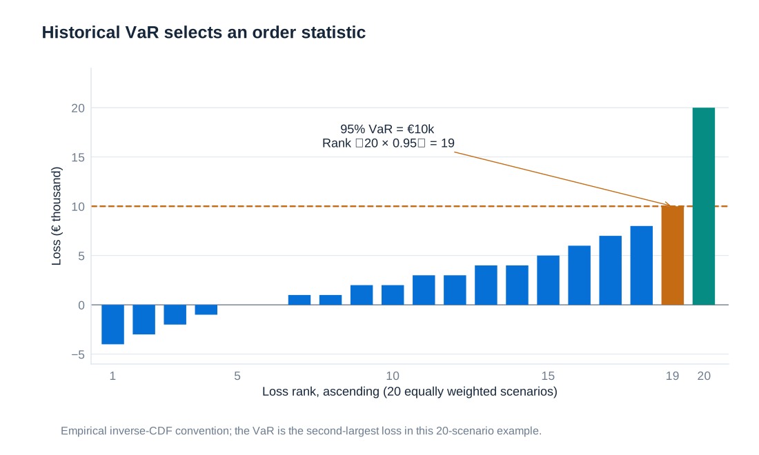
Historical simulation does not require a specific parametric density, but it still assumes that the chosen history is informative about future shocks. It retains only the skewness, tails and dependence present in that sample. A short window may omit a crisis; a long window may mix obsolete regimes with current conditions. Structural breaks, new instruments and missing price histories can make the sample unreliable. Full revaluation captures nonlinear option responses; a historical simulation using only delta approximations does not automatically capture gamma merely because its scenarios are historical.
Variance–covariance and delta–gamma approaches
Let be a vector of risk-factor changes, with mean vector and covariance matrix . Let be the monetary sensitivity of portfolio profit to factor , so the first-order approximation is . For percentage-return factors, is a currency exposure per unit decimal return; for rate changes, it must match the rate unit. The variance is:
The diagonal elements of are factor variances; off-diagonal elements are covariances. If the factor vector is jointly multivariate normal, a linear combination is normal and the delta-normal VaR is . Marginal normality of each factor alone is insufficient: their joint dependence must be specified. Correlations are a major source of diversification, and changes in them can materially alter the result even if each volatility stays fixed.
For an illustrative two-position portfolio, let each position have one-day profit standard deviation EUR 100,000 and correlation 0.5. Portfolio standard deviation is . With zero expected profit, 99% normal VaR is approximately EUR 402,935. If correlation becomes 1, standard deviation rises to EUR 200,000 and VaR to EUR 465,270. The diversification benefit is conditional on dependence, not a permanent property of holding two positions.
A delta–gamma approximation adds the Hessian matrix of second derivatives: . Even when is jointly normal, this quadratic profit is generally not normal. Its quantile may require simulation or a specialised quadratic-form method. Adding gamma and then mechanically multiplying a standard deviation by 2.3263 does not generally produce an exact 99% quantile.
The delta-normal method is fast, transparent and useful for hedge comparisons because it has a closed-form calculation without Monte Carlo sampling error. Its limitations are the linear valuation approximation and the chosen distribution, covariance estimates and factor mapping. Eliminating simulation error does not eliminate parameter uncertainty or model risk. For large option books, fast approximations should be compared with full revaluation under meaningful stresses.
Monte Carlo simulation and the source of simulation error
Monte Carlo simulation specifies a joint probability model, generates many scenarios, values the current portfolio in each and reads the desired quantile from the simulated losses. A run of 10,000 scenarios is a possible starting point, not an assurance of accurate extreme-tail estimates. The method may use normal, heavy-tailed, skewed, jump or other models where justified; normality is not inherent in simulation.
For a multivariate normal example, draw independent standard normal variables , choose a matrix satisfying , and set . A Cholesky factor can be used when the covariance matrix is suitable. Independent draws for the components of do not imply independent simulated factors: the matrix transformation introduces the chosen dependence. Each scenario then feeds a consistent pricing model, producing a monetary portfolio loss.
Full pricing can represent nonlinear options, while path-dependent instruments require simulated paths rather than only terminal shocks. A scenario distribution and valuation model must also be kept conceptually separate: market-risk probabilities usually describe real-world future changes, while option values within each scenario may be calculated using risk-neutral pricing assumptions. Confusing the two probability roles can distort the loss distribution.
Simulation error remains because the scenario sample is finite. At 99% confidence, 10,000 draws leave only about 100 observations beyond the estimated threshold. Results can be checked across independent runs or with appropriate uncertainty estimates, and more draws may improve precision. A fixed random seed supports reproducibility but does not establish accuracy. Parameter misspecification, missing factors and wrong pricing persist even with millions of scenarios. The computational flexibility must therefore be matched by calibration, validation and clear documentation.
Volatility clustering, weighting, EWMA and GARCH
Financial return distributions often have heavier tails and asymmetry relative to a fitted normal distribution. Large absolute returns also tend to cluster: turbulent periods follow turbulent periods, and quiet periods follow quiet periods. A single unconditional standard deviation can consequently describe neither regime well. Empirical histograms and return histories are evidence about these features, not a proof that one alternative model will always forecast them correctly.
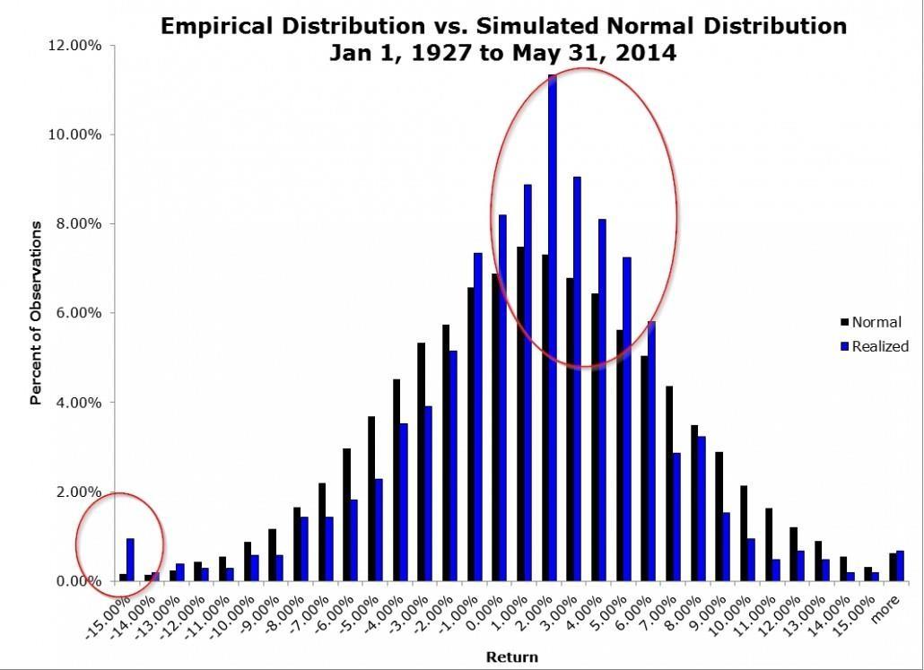
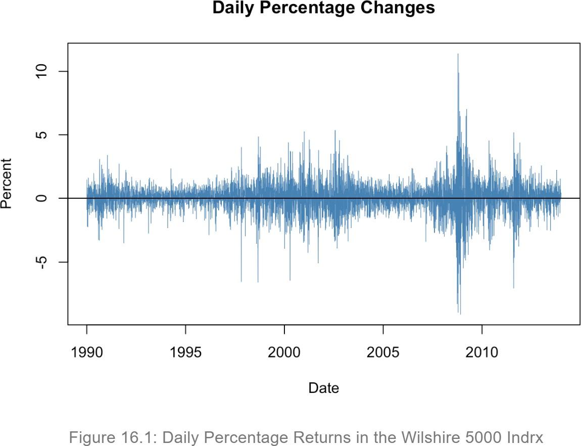
Historical weighting gives recent observations greater influence. For an exponentially weighted moving average, or EWMA, a zero-mean innovation updates the variance forecast as:
A smaller responds faster to new observations and forgets earlier shocks more quickly. In an illustrative daily model with , current volatility 1% and latest innovation 3%, the next variance is . The next volatility is therefore about 1.2166%, not the weighted average of 1% and 3%. Variances, rather than standard deviations, are being updated.
Ignoring the finite-sample initialisation term, an observation periods back receives weight . At 0.94, the most recent twenty observations carry about 70.99% of the infinite-history weight, and the most recent fifty about 95.47%. A finite window requires consistent normalisation or retention of the initial-variance contribution. Weighted historical quantiles use cumulative scenario weights rather than the unweighted rank formula.
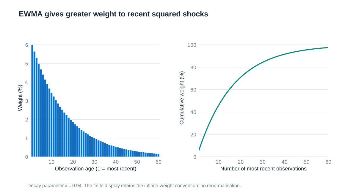
A GARCH(1,1) model adds a constant and separates the shock and persistence coefficients:
For a finite constant unconditional variance in the usual model, , giving . With illustrative values , , , current variance 0.0001 and innovation 0.03, the next variance is 0.000164 and volatility about 1.2806%. The long-run variance is 0.0001. EWMA corresponds to the special zero-intercept recursion with shock and persistence coefficients summing to one, so it does not have this finite mean-reverting variance formula.
These methods forecast conditional volatility; they do not automatically remove skewness, jumps or fat tails from standardised innovations. Filtered historical simulation rescales historical standardised shocks by current volatility forecasts, with dependence and multivariate rescaling treated consistently. A model that adapts rapidly to volatility can still underestimate a new regime, and its forecasts should be compared with stresses that are not mechanically limited to recent experience.
Tail severity, Expected Shortfall and diversification
VaR can remain nearly unchanged when a loss beyond the chosen quantile becomes much larger. Selling a far out-of-the-money put illustrates the problem: most days may show small premium income or modest valuation changes, while a collapse of the underlying creates a severe loss. The premium is compensation for an exposure, not evidence that the exposure has disappeared. A sample without a crash can report very low VaR for a strategy whose economic tail is substantial.
For an integrable loss distribution, Expected Shortfall averages quantiles in the worst fraction:
With a continuous distribution this equals under the usual tail conditions. For a discrete distribution with probability mass at the VaR threshold, the simple conditional expectation can be wrong: the quantile-average definition includes the appropriate fraction of the threshold mass. In the twenty-scenario illustration, 95% VaR is 10 thousand and ES is 20 thousand because the worst 5% is one observation.
For normal loss , , where is the standard normal density. With mean zero and unit standard deviation, 99% VaR is about 2.3263 and ES about 2.6652. ES describes severity beyond the quantile; it is still model-dependent and is not a worst-case bound.
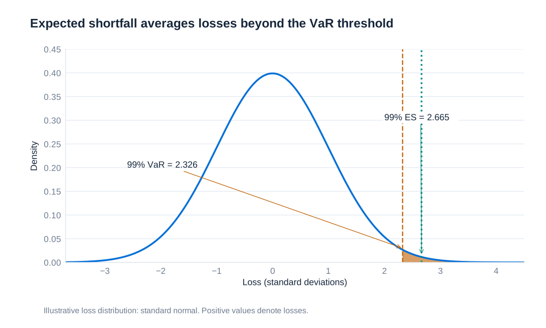
VaR is not subadditive for every loss distribution. Consider two independent positions, each losing 100 with probability 4% and zero otherwise. Each has 95% VaR zero because a zero loss occurs with probability 96%. Together, the probability of no loss is , so the combined 95% VaR is 100, exceeding the sum of the standalone VaRs. This counterexample does not imply that diversification always increases VaR; it shows that VaR does not universally reward it. ES is subadditive for integrable losses and, together with monotonicity, positive homogeneity and cash-translation behaviour, is a coherent risk measure.
Quiet samples, carry trades and the Niederhoffer case
A carry trade borrows in a low-interest-rate currency and invests in a higher-interest-rate currency without fully eliminating exchange-rate exposure. An illustrative USD-funded Thai-baht investment earning 12% while funding costs 6% appears to earn a 6-percentage-point spread if the exchange rate is unchanged. The interest differential is not a risk-free arbitrage. If the baht value in dollars falls 20% over the year, one borrowed dollar produces dollars of investment proceeds but requires 1.06 dollars of repayment, a loss of 0.164 dollars before other costs.
Thailand allowed the baht to float on 2 July 1997, after pressure on its exchange-rate arrangement. This date must be distinguished from the sharp US equity-market fall on 27 October 1997 and from the timing of individual fund losses. A previously stable exchange rate can produce a low historical volatility estimate until the regime changes. A narrow calibration window may therefore mistake the absence of a past break for the absence of future currency risk.
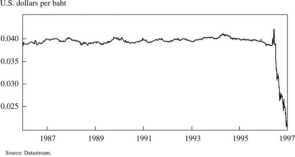
Victor Niederhoffer’s 1997 fund collapse provides a related warning about strategies with strong historical returns and severe exposure to exceptional market moves. It should not be reduced to a single elementary currency carry calculation: option exposures, leverage, market movements and funding pressures can interact. A high historical Sharpe ratio, which compares excess return with volatility, may be uninformative about rare losses when the observation window contains mainly premium income or a stable regime.
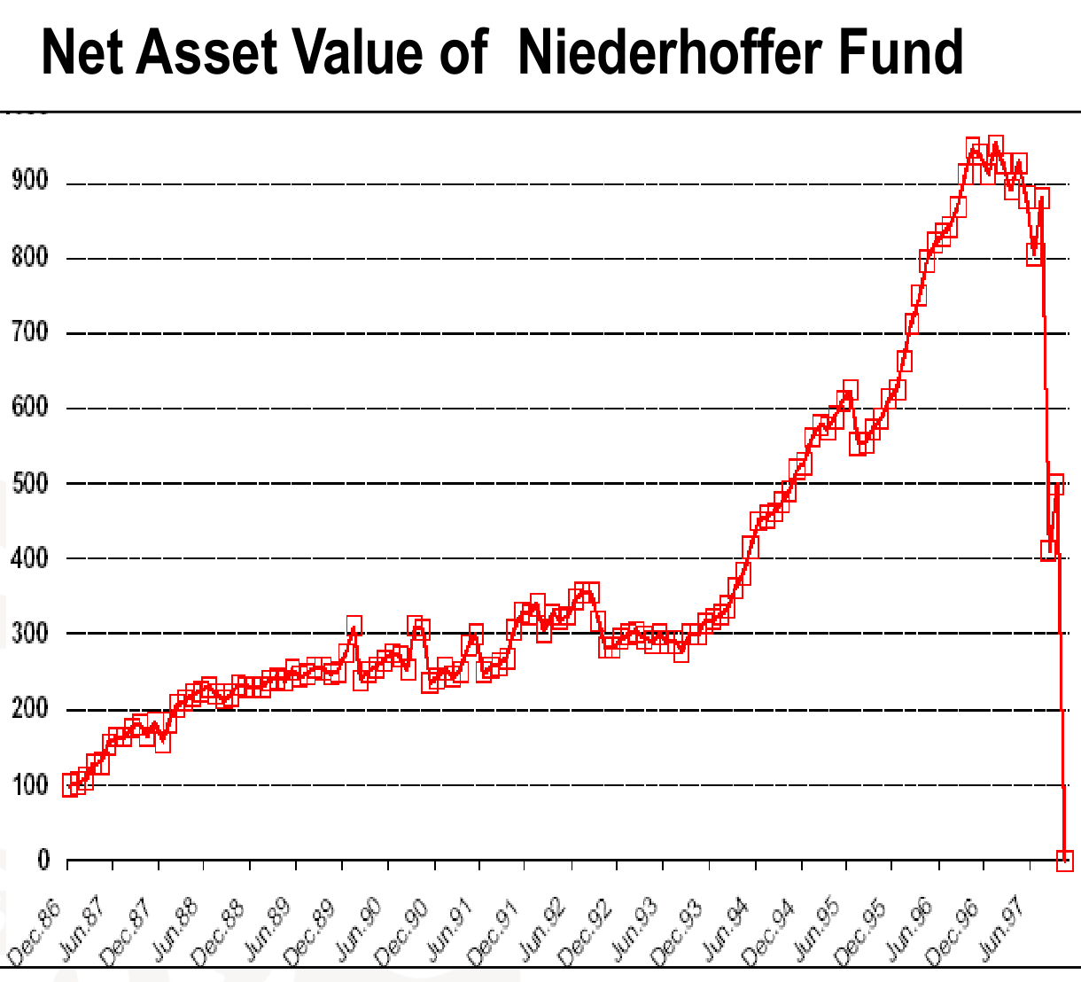
The general problem is model risk at several levels: volatility and correlation estimates are uncertain; the assumed distribution may miss jumps or tail dependence; and valuation may be inaccurate precisely in stressed markets. Sensitivity to alternative windows, distributions and correlations should be visible. Stress testing asks how a plausible severe scenario would affect the portfolio even if the fitted probability model assigns it little weight. Reverse stress testing starts from an unacceptable loss and asks which combinations of events could produce it.
Historical source: IMF, Thailand stand-by credit release (1997).
Backtesting, implementation controls and the London Whale
Backtesting compares a forecast made using information available at the time with the subsequent outcome. For a 99% daily VaR, the exception indicator is . A well-calibrated model should have an appropriate exception rate, but frequency alone is insufficient: exceptions clustered during crises reveal conditional misspecification even if the long-run count looks acceptable. Actual trading profit and hypothetical profit on an unchanged portfolio answer different validation questions because new trades, fees and intraday decisions can affect realised results.
The London Whale episode at JPMorgan in 2012 illustrates why implementation and governance matter alongside the statistical formula. The US Senate investigation reported that a new CIO model reduced measured VaR by approximately 50% on introduction, while the positions had not thereby become safer. It identified manual operations, calculation and implementation errors and weaknesses in model review. The broader case also involved risk-limit responses and valuation controls. Attributing the entire loss to a single typographical error would obscure these interacting failures.
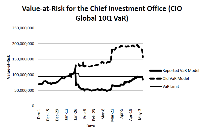
Independent validation should examine whether mathematical specifications are implemented faithfully, compare old and new models on the same positions, reconcile input data and review abrupt risk-number reductions. A lower estimate is not itself evidence of an improved model. Material model changes need a documented economic explanation, independent challenge and clear treatment of existing limits. Sensitivity analysis, stress results and position concentrations should remain available even when a preferred VaR model produces a reassuring number.
Investigation: US Senate, JPMorgan Chase Whale Trades report (2013).
Time horizons, liquidity and the evolution of market-risk regulation
If daily profit increments are independent and identically distributed with mean and variance , their sum over days has mean and variance . With normal increments and stable exposures:
When the mean is negligible, ten-day normal VaR is approximately times one-day VaR, not ten times. Independence and identical distributions alone establish variance scaling when variance exists; they do not make every distribution’s quantile scale exactly with the square root of time. Serial dependence, changing volatility, nonlinear valuation, jumps, rebalancing and liquidation costs can invalidate the shortcut. A position that cannot be sold quickly also remains exposed beyond a nominal one-day reporting horizon.
J.P. Morgan publicly launched RiskMetrics in 1994. The Basel Committee’s 1996 Market Risk Amendment introduced a framework permitting standardised market-risk capital calculations and approved internal models. Post-crisis reforms included the 2009 Basel 2.5 changes and stressed VaR. The Fundamental Review of the Trading Book, or FRTB, subsequently centred the internal-model framework on stressed ES and liquidity risk. The ECB’s Targeted Review of Internal Models, or TRIM, is a separate supervisory review initiative; interest-rate risk in the banking book also has its own supervisory framework rather than simply being absorbed into trading-book VaR.
The Basel market-risk standard uses 97.5% one-tailed ES and a ten-day base horizon, with specified liquidity-horizon categories extending to 120 days. The following mapping summarises the risk-factor categories in that framework; it describes the standard, not a claim that every jurisdiction applies every provision on an identical implementation date. IG denotes investment grade and HY high yield.
| Risk-factor category | Horizon |
|---|---|
| Interest rates: specified currencies and a bank’s domestic currency | 10 |
| Interest rates: other currencies | 20 |
| Interest-rate volatility and other interest-rate factors | 60 |
| Sovereign credit spreads: IG | 20 |
| Sovereign credit spreads: HY | 40 |
| Corporate credit spreads: IG | 40 |
| Corporate credit spreads: HY | 60 |
| Credit-spread volatility and other credit-spread factors | 120 |
| Large-cap equity prices | 10 |
| Small-cap equity prices and large-cap equity volatility | 20 |
| Small-cap equity volatility and other equity factors | 60 |
| FX rates: specified currency pairs | 10 |
| FX rates: other currency pairs | 20 |
| FX volatility and other FX factors | 40 |
| Energy and carbon-emissions prices | 20 |
| Precious and non-ferrous metal prices | 20 |
| Other commodity prices | 60 |
| Energy, carbon-emissions, precious and non-ferrous metal volatility | 60 |
| Other commodity volatility and other commodity factors | 120 |
The specified interest-rate currencies include EUR, USD, GBP, AUD, JPY, SEK and CAD, together with the bank’s domestic currency. Exact FX-pair eligibility and supervisory adjustments require the framework’s definitions. Liquidity-adjusted ES aggregates exposures assigned to different horizons; it is not obtained by multiplying the entire portfolio by its longest horizon. Modelling the availability and quality of market observations is also necessary, because stale or sparse prices can make apparently precise factors unsuitable for the normal modelling process.
Regulatory references: Basel Framework MAR33; Basel Committee, market-risk capital requirements (2019).
Model heterogeneity and the limits of a single number
Even when institutions value the same positions, different data windows, dependence assumptions, pricing approximations and implementation choices can generate materially different capital estimates. The Basel Committee’s 2013 regulatory consistency assessment reported the following results for a common diversified test portfolio. The figures are historical model-comparison evidence, not current capital requirements for an investor’s portfolio.
| Statistic across models | Reported value |
|---|---|
| Minimum | EUR 13,414,208 |
| Maximum | EUR 34,165,014 |
| Median | EUR 17,781,481 |
| Mean | EUR 20,521,469 |
| Standard deviation | EUR 6,344,392 |
| Standard deviation divided by mean | 31%, rounded |
The maximum is more than twice the minimum. This dispersion is a reason to investigate model choices, not proof that the smallest or largest estimate is automatically correct. Regulatory capital incentives can create pressure to favour low measured risk, making independent governance especially important. Harmonised definitions, validation, benchmarking and credible standardised alternatives help constrain unjustified differences.
A useful risk report therefore places VaR and ES beside stress losses, sensitivities, liquidity assumptions, concentrations and model limitations. VaR supplies a common threshold language; ES adds tail severity; neither removes the need to understand the positions. The quality of market data, valuation, implementation and escalation determines whether the resulting numbers support decisions or merely give false precision.
Historical comparison: Basel Committee, analysis of market-risk weighted assets (2013).
7. Credit Risk: Measurement, Ratings and Portfolio Management
Credit risk arises whenever one party depends on another party to honour an obligation. A bank's loan book is the obvious example, but the same exposure appears in trade receivables, credit cards, leasing, instalment purchases and derivatives. A traveller who pays for an airline ticket before departure extends credit to the airline; a telecommunications provider that supplies a handset before collecting all monthly payments extends credit to the customer. Bond investors, landlords and suppliers therefore face different versions of the same problem: promised cash flows may arrive late, arrive only partly or never arrive.
Default, deterioration and the definition of loss
A default can involve insolvency, a material payment that remains overdue, or a distressed restructuring that reduces the creditor's economic claim. Regulatory definitions also consider whether the borrower is unlikely to pay without enforcement of collateral. A 90-day past-due trigger is widely used, but its precise application depends on the applicable framework, materiality thresholds and exposure category. Legal bankruptcy is consequently neither the only default event nor a necessary condition for every credit loss. A rating of D or a non-performing-loan designation communicates a default-related status, whereas a performing loan can already have substantial credit risk.
Credit deterioration matters before default. A rating downgrade, an increase in an internally estimated probability of default or a widening market credit spread can reduce the present value of a claim while all payments remain current. Default risk, migration risk and spread risk overlap economically but are not interchangeable measurement categories. A trading portfolio may recognise spread changes through market-risk measures, while a banking-book portfolio uses default and impairment measures. Calling an exposure “credit risk” does not by itself determine its accounting treatment or its prudential classification.
Measurement must therefore specify the horizon, valuation basis and aggregation level. The eventual unpaid amount on one loan is different from the present market-value loss on a bond, and neither is the same as the unexpected loss of a diversified portfolio. Internal ratings and external ratings describe credit quality; expected loss describes a mean monetary shortfall; economic capital describes a tail buffer; and risk-weighted assets are a regulatory denominator used to determine capital requirements. Treating these quantities as substitutes obscures the decision each one supports.
PD, LGD and EAD
The three central components are probability of default, or PD; exposure at default, or EAD; and loss given default, or LGD. PD is the probability that a specified default event occurs over a specified horizon. EAD is the amount exposed when default occurs, including relevant drawings or accrued amounts rather than necessarily today's outstanding principal. LGD is the fraction of that exposure lost after allowing for recoveries and the associated costs and timing. If recovery is immediate, costless and measured on the same exposure basis, LGD equals one minus the recovery rate.
For deterministic EAD and an appropriately defined conditional mean LGD, the familiar one-period relation is
PD and LGD enter as decimals, and EAD is a currency amount, so expected loss has the same currency unit. Consider a €100 loan with a 10% probability of default and an expected recovery of €50 if default occurs. The conditional loss is €50, LGD is 50%, and expected loss is euros. The borrower does not pay an “expected” €5 loss in every outcome: the simplified distribution has a €50 loss with probability 10% and no loss with probability 90%.
| Outcome | Probability | Credit loss | Contribution to expected loss |
|---|---|---|---|
| No default | 90% | €0 | €0 |
| Default with €50 recovery | 10% | €50 | €5 |
| Total | 100% | Outcome-dependent | €5 |
The factorisation needs care when exposure and recovery are random. With a default indicator , the general object is , not automatically . A borrower may draw unused credit immediately before default, while collateral values fall during the same downturn. A revolving facility with €60 drawn and €40 undrawn, for example, has EAD of €80 if the assumed conversion factor on the undrawn portion is 50%. That is a modelling assumption, not a universal conversion factor. Legal enforceability, collateral liquidity and recovery costs can make LGD materially higher than the apparent shortfall between loan principal and today's collateral valuation.
For a multi-year exposure, losses at different dates and in different economic scenarios must be combined without counting the same default repeatedly. Let be the marginal probability of first default in year under scenario , the scenario probability and a discount factor consistent with the measurement purpose. A simplified representation is
The scenario weights sum to one. The loss severity should incorporate the timing of recoveries consistently, so discounting is not applied twice. Accounting expected credit loss, a market price and prudential expected loss can use different probability concepts, horizons and prescribed inputs. Sharing the labels PD, LGD and EAD does not make the resulting estimates identical.
Impairment, write-offs and fair-value losses
Under the general IFRS 9 impairment model, Stage 1 ordinarily recognises 12-month expected credit losses. This is the lifetime cash shortfall associated with defaults that could occur in the next 12 months, not merely cash payments missed during those months. A significant increase in credit risk moves an exposure to Stage 2 and lifetime expected credit losses. Stage 3 concerns credit-impaired assets and also uses lifetime expected losses; interest revenue is generally calculated on the net carrying amount. Special approaches and exceptions exist, so these three stages describe the general model rather than every financial asset.
An impairment charge changes the allowance and profit or loss; it does not necessarily mean that the borrower has already defaulted. A write-off directly reduces the gross carrying amount when there is no reasonable expectation of recovering all or part of the asset. It need not wait for the formal end of insolvency proceedings. If the loss was already fully provided for, the later write-off mainly uses the existing allowance rather than creating the same expense a second time. Changes in fair value are a separate channel for instruments measured at fair value.
The US current expected credit losses model, CECL, belongs to US GAAP and is not another name for IFRS 9. For financial assets within its amortised-cost scope, it generally recognises lifetime expected credit losses from initial recognition. Both systems are forward-looking, but their recognition frameworks differ. Comparing banks across accounting systems therefore requires more than comparing the words “expected loss” in their reports.
Accounting references: ESRB comparison of European and US expected-loss approaches; IFRS 9 impairment review, including write-offs; Federal Reserve CECL guidance.
Expected loss, unexpected loss and economic capital
At portfolio level, loss is a random variable . Its mean describes expected loss; a quantile describes a tail outcome. Define as the smallest loss level reached with cumulative probability at least . One common economic-capital convention is , the tail loss above the mean. In this manual, unexpected loss is the standard deviation . Some institutions use that term for quantile-minus-mean instead; stating the convention is essential because these quantities differ.
Expected credit losses are ordinarily considered in pricing, provisions and operating income. Capital provides capacity to absorb adverse deviations and other risks. The economic-capital confidence level is a management choice linked to the institution's solvency objective; 99%, 99.9% and 99.98% are not interchangeable universal standards. Regulatory capital is determined by a separate set of rules. Risk-weighted assets, or RWA, are neither cash losses nor capital itself: a capital ratio applies a required percentage to the RWA denominator.
Consider an illustrative portfolio of 100 independent loans, each with EAD €1 million, one-year PD 2% and deterministic LGD 45%. The number of defaults is binomial with parameters 100 and 0.02, and total loss is million euros. Expected loss is €0.9 million. The standard deviation is million euros. The exact 99.9% loss quantile is seven defaults, or €3.15 million; economic capital is therefore €3.15 million minus €0.9 million, giving €2.25 million. The quantile is determined from the binomial cumulative distribution, not a normal approximation. This stylised example isolates diversification across independent borrowers; real portfolios can have much more severe tails because defaults are dependent.
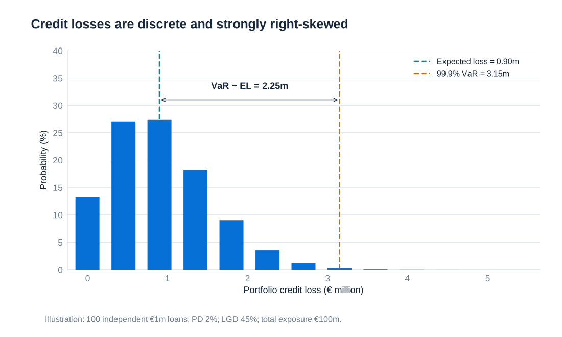
Credit risk frequently dominates banks' risk allocations, but the share depends on business model and measurement basis. Historical illustrations report credit risk as 49.6% of €77 billion of economic capital for five large German banks, with approximately €38 billion allocated to credit risk; total credit exposure was €1,938 billion and retail and small businesses represented 29.3%. Another historical savings-bank illustration allocates approximately 78% to credit risk, 20% to market risk and 1% to operational risk, with rounding. Such figures illustrate materiality rather than providing a current banking-sector benchmark, and economic-capital allocations must not be relabelled as RWA.
The economic logic of the IRB capital formula
The internal ratings-based approach, IRB, links regulatory credit capital to PD, LGD, EAD, maturity and a prescribed asset-correlation function. Its underlying asymptotic single-factor model assumes a highly granular portfolio: individual borrower shocks diversify, but a common systematic factor remains. A severe state of that factor raises the conditional default rate. For an ordinary non-defaulted corporate exposure, the core expression can be written
Here is the standard normal cumulative distribution function, its inverse, the prescribed asset correlation, effective maturity in years, and a capital ratio before multiplying by EAD. For the basic corporate correlation function, before applicable adjustments,
The square root on the systematic-factor loading is essential. The term is a conditional stressed loss rate; subtracting removes expected loss from the core unexpected-loss component. The factor 12.5 converts capital into RWA at an 8% reference capital ratio. RWA are consequently not equal to the 99.9% portfolio loss quantile. The maturity adjustment changes the charge according to effective maturity; the ordinary framework commonly constrains maturity between one and five years, with specific exceptions. Asset classes, smaller-company adjustments and certain financial-institution exposures require their own prescribed treatment.
The legacy Basel II scaling multiplier 1.06 has been removed from the revised Basel framework. Likewise, the old 0.03% PD floor is not a universal current rule: the revised framework generally uses 0.05% for corporate and bank exposures, with sovereign exceptions and distinct retail provisions. A zero observed default count does not establish zero credit risk. Long-run calibration, data requirements, conservatism and applicable floors address sparse-default samples.
Basel standards are implemented through jurisdiction-specific law. In the EU, CRR3 introduced the final Basel III package from 2025, including an output floor phased from 50% towards 72.5% in 2030. This limits the reduction in aggregate capital requirements obtainable from internal models relative to standardised calculations; it is not a floor on each individual loan's PD. Sovereign exposures are not universally assigned zero risk weight: preferential treatment depends on the applicable approach and conditions, including relevant domestic-currency provisions. Regulatory zero weight would in any event not mean economic impossibility of default.
Prudential references: Basel CRE31 risk-weight functions; CRE32 risk components; removal of the 1.06 multiplier; Regulation (EU) 2024/1623; EU output-floor transition.
Market-implied default probabilities
Credit assessment can use financial statements, management information, payment histories, external ratings and market prices. Bond and CDS prices provide forward-looking information, but they price risk under a risk-neutral measure. A risk-neutral PD is a valuation input that reproduces market prices under appropriate discounting; it is not automatically the physical frequency with which comparable borrowers will default.
Consider one-year zero-coupon bonds with face value €100. The risk-free yield is 5%, giving a price of euros. A risky bond has a promised yield of 10%, giving a price of euros. Suppose its maturity payoff is €100 without default and €50 after default. With risk-neutral default probability ,
The promised 10% yield is not the expected realised return. Risk-neutral expected payoffs discounted at 5% reproduce the price. The physical PD may be lower when investors require compensation for systematic default risk, but there is no universal fixed difference between the two probabilities. Liquidity, risk aversion, taxes, contractual features and market frictions can also affect spreads, so a simple spread-to-PD conversion can misattribute non-default components to default risk.
Historical bond spreads widen markedly in downturns, especially for speculative-grade debt. That movement can reflect worse expected cash flows, lower recovery prospects, a higher price of bearing risk and deteriorating market liquidity at the same time. A widening spread is therefore a warning signal, not a direct observation of a uniquely identified physical PD.
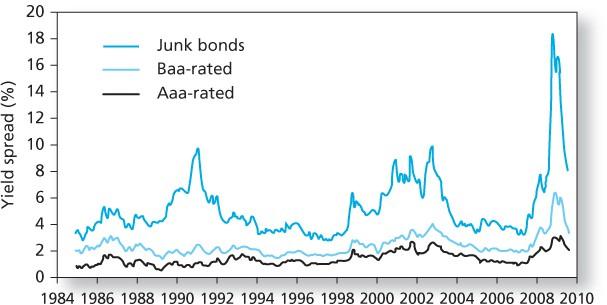
Structural credit risk: the Merton model
A structural model connects default to the value of the borrower's assets. In the simplest Merton setting, the firm has asset value and one zero-coupon debt obligation with face value due at time . Default occurs at maturity when . With limited liability, equity receives , so equity is a call option on the firm's assets. Debt receives , equivalently a risk-free payment of minus a put-option payoff.
Under risk-neutral geometric Brownian motion, constant asset volatility , a constant continuously compounded risk-free rate and no asset payouts, equity value is
The physical default probability replaces the risk-neutral drift with the physical expected asset return in the distance-to-default expression. Higher leverage reduces the distance between asset value and the debt threshold; higher asset volatility increases exposure to downside states. Because corporate assets are not usually traded directly, implementation must infer asset value and volatility from observed securities and balance-sheet information. The assumption of default only at a single maturity is restrictive: real firms have several debt maturities, covenants, liquidity constraints and possible early default.
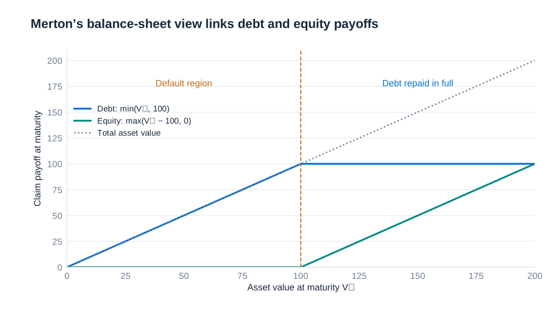
Structural models and statistical accounting-score models should not be confused. A market-based expected-default-frequency approach can use structural intuition and empirical calibration, while a private-firm score based on accounting ratios estimates risk statistically. The product name or the rating provider does not establish which model is being used. The relevant questions are its inputs, target event, horizon, probability measure and validation performance.
External ratings and their meaning
External ratings order issuers or obligations by creditworthiness. The investment-grade boundary is BBB− for S&P and Fitch and Baa3 for Moody's; lower categories are speculative grade. A notch is one step within this ordered scale. An issuer rating and an issue rating can differ because a particular claim has collateral, guarantees or subordination. Rating symbols also have agency-specific definitions; a cross-agency correspondence is a broad comparison, not a guarantee that the underlying risks or methodologies are identical.
| S&P | Fitch | Moody’s | Broad category |
|---|---|---|---|
| AAA | AAA | Aaa | Investment grade |
| AA+ | AA+ | Aa1 | Investment grade |
| AA | AA | Aa2 | Investment grade |
| AA− | AA− | Aa3 | Investment grade |
| A+ | A+ | A1 | Investment grade |
| A | A | A2 | Investment grade |
| A− | A− | A3 | Investment grade |
| BBB+ | BBB+ | Baa1 | Investment grade |
| BBB | BBB | Baa2 | Investment grade |
| BBB− | BBB− | Baa3 | Investment grade |
| BB+ | BB+ | Ba1 | Speculative grade |
| BB | BB | Ba2 | Speculative grade |
| BB− | BB− | Ba3 | Speculative grade |
| B+ | B+ | B1 | Speculative grade |
| B | B | B2 | Speculative grade |
| B− | B− | B3 | Speculative grade |
| CCC+ | CCC+ | Caa1 | Speculative grade |
| CCC | CCC | Caa2 | Speculative grade |
| CCC− | CCC− | Caa3 | Speculative grade |
| CC | CC | Ca | Speculative grade |
| C | C | C | Speculative grade |
At the bottom of the scale, S&P uses default-related designations including D and SD, and Fitch distinguishes D and RD. Moody's does not use D as an ordinary long-term rating category; its C category can include obligations in default. Rating methodologies also differ in the relative emphasis placed on default likelihood, loss severity and the credit characteristics of particular obligations. “Through the cycle” describes an effort to look beyond temporary conditions, not a promise that a rating never changes during a cycle or corresponds to one permanently fixed one-year PD.
From business and financial risk to an anchor rating
A corporate rating combines business risk with financial risk. Business risk reflects country and industry conditions and the firm's competitive position. Financial risk draws on cash generation, debt burden and coverage ratios after accounting adjustments that improve comparability. An initial anchor is then modified for diversification, capital structure, financial policy, liquidity, management and governance, and comparable-rating analysis. Group or government support can change the final issuer assessment relative to the stand-alone credit profile.
In the historical process example, country risk is scored 2 (low), industry risk 4 (moderately high), their combined country-and-industry assessment is 4, and competitive position is 3 (satisfactory). The resulting business-risk profile is 3 (satisfactory). These are category scores within that methodology, not probabilities or quantities to average mechanically. The financial assessment and later modifiers are still needed before determining an issuer rating.
A historical Daimler illustration shows why reported debt is not necessarily the debt figure used in credit analysis. Operating leases and post-retirement obligations increase adjusted obligations, while surplus cash and financing-business adjustments can reduce the industrial debt measure. The following historical figures are in EUR millions. A denotes actual data; P and E denote projected or estimated columns. Repeated projected values are retained as stated, not interpreted as realised later outcomes.
| Adjustment | 2012A | 2013A | 2014P | 2015E | 2016E |
|---|---|---|---|---|---|
| Reported debt | 76,251 | 77,738 | 77,738 | 77,738 | 77,738 |
| Operating leases | 1,672 | 1,501 | 1,501 | 1,501 | 1,501 |
| Post-retirement benefit obligations | 10,324 | 9,109 | 9,109 | 9,109 | 9,109 |
| Less surplus cash | −12,837 | −13,848 | −13,848 | −13,848 | −13,848 |
| Less captive-finance adjustment | −64,272 | −67,497 | −67,497 | −67,497 | −67,497 |
| Other adjustments | 120 | 454 | 454 | 454 | 454 |
| Fully adjusted debt | 11,258 | 7,457 | 7,457 | 7,457 | 7,457 |
The adjusted debt amount is approximately €11,258 million for 2012 and €7,457 million for the later columns. Small reconciliation differences can arise from the rounding of the individual displayed adjustments. The accounting perimeter matters: separating captive finance debt from industrial debt does not make those finance-company obligations disappear from the consolidated group or remove their economic risks.
The next historical grid translates ratios into financial-risk categories. FFO is funds from operations, EBITDA is earnings before interest, tax, depreciation and amortisation, OCF is operating cash flow, FOCF is free operating cash flow, and DCF here means discretionary cash flow, not discounted cash flow. The ratios are agency-adjusted measures. Thresholds depend on methodology and industry; this 2014-era grid explains the rating process and is not a current universal rulebook.
| Financial risk | FFO/debt (%) | Debt/EBITDA (×) | FFO/cash interest (×) | EBITDA/interest (×) | OCF/debt (%) | FOCF/debt (%) | DCF/debt (%) |
|---|---|---|---|---|---|---|---|
| Minimal | >60 | <1.5 | >13 | >15 | >50 | >40 | >25 |
| Modest | 45–60 | 1.5–2 | 9–13 | 10–15 | 35–50 | 25–40 | 15–25 |
| Intermediate | 30–45 | 2–3 | 6–9 | 6–10 | 25–35 | 15–25 | 10–15 |
| Significant | 20–30 | 3–4 | 4–6 | 3–6 | 15–25 | 10–15 | 5–10 |
| Aggressive | 12–20 | 4–5 | 2–4 | 2–3 | 10–15 | 5–10 | 2–5 |
| Highly leveraged | <12 | >5 | <2 | <2 | <10 | <5 | <2 |
Combining business and financial assessments gives the following historical anchor matrix. Lower-case symbols identify intermediate analytical anchors. A satisfactory business profile with minimal financial risk produces an a/a− anchor in this example; weak liquidity or an aggressive financial policy can still alter the eventual rating. A matrix cannot substitute for assessment of the definitions underlying its rows and columns.
| Business risk | Minimal | Modest | Intermediate | Significant | Aggressive | Highly leveraged |
|---|---|---|---|---|---|---|
| Excellent | aaa/aa+ | aa | a+/a | a− | bbb | bbb−/bb+ |
| Strong | aa/aa− | a+/a | a−/bbb+ | bbb | bb+ | bb |
| Satisfactory | a/a− | bbb+ | bbb/bbb− | bbb−/bb+ | bb | b+ |
| Fair | bbb/bbb− | bbb− | bb+ | bb | bb− | b |
| Weak | bb+ | bb+ | bb | bb− | b+ | b/b− |
| Vulnerable | bb− | bb− | bb−/b+ | b+ | b | b− |
Default probabilities across horizons
A rating becomes more useful for measurement when it is connected to a clearly defined default frequency and horizon. The historical table below reports average cumulative corporate default rates by initial rating, measured in percent, over the 1981–2014 observation period. A cumulative rate includes defaults occurring at any time before the stated horizon. The rows are historical averages for different initial-rating cohorts; they are not forecasts for a current issuer and should not be combined as though every category had the same number of observations.
| Initial rating | 1 year | 2 years | 3 years | 4 years | 5 years | 6 years | 7 years | 8 years | 9 years | 10 years | 11 years | 12 years | 13 years | 14 years | 15 years |
|---|---|---|---|---|---|---|---|---|---|---|---|---|---|---|---|
| AAA | 0.00 | 0.03 | 0.14 | 0.24 | 0.36 | 0.47 | 0.53 | 0.61 | 0.67 | 0.74 | 0.77 | 0.80 | 0.84 | 0.91 | 0.98 |
| AA | 0.02 | 0.07 | 0.13 | 0.24 | 0.35 | 0.46 | 0.56 | 0.65 | 0.73 | 0.82 | 0.90 | 0.97 | 1.05 | 1.12 | 1.19 |
| A | 0.07 | 0.16 | 0.27 | 0.41 | 0.57 | 0.75 | 0.95 | 1.13 | 1.32 | 1.51 | 1.69 | 1.84 | 2.00 | 2.15 | 2.32 |
| BBB | 0.20 | 0.57 | 0.96 | 1.46 | 1.95 | 2.43 | 2.84 | 3.26 | 3.66 | 4.06 | 4.49 | 4.84 | 5.17 | 5.50 | 5.84 |
| BB | 0.76 | 2.35 | 4.23 | 6.06 | 7.71 | 9.28 | 10.59 | 11.75 | 12.80 | 13.74 | 14.52 | 15.18 | 15.75 | 16.24 | 16.77 |
| B | 3.88 | 8.80 | 12.97 | 16.22 | 18.70 | 20.72 | 22.37 | 23.69 | 24.82 | 25.91 | 26.82 | 27.57 | 28.26 | 28.88 | 29.49 |
| CCC/C | 26.38 | 35.58 | 40.67 | 43.77 | 46.28 | 47.24 | 48.27 | 49.06 | 50.03 | 50.73 | 51.28 | 51.94 | 52.72 | 53.38 | 53.38 |
| Investment grade | 0.11 | 0.29 | 0.50 | 0.76 | 1.03 | 1.29 | 1.54 | 1.78 | 2.01 | 2.24 | 2.46 | 2.65 | 2.83 | 3.01 | 3.20 |
| Speculative grade | 3.87 | 7.58 | 10.79 | 13.39 | 15.49 | 17.23 | 18.69 | 19.90 | 20.98 | 21.97 | 22.79 | 23.49 | 24.13 | 24.68 | 25.22 |
| All rated | 1.50 | 2.95 | 4.23 | 5.31 | 6.20 | 6.97 | 7.62 | 8.18 | 8.68 | 9.15 | 9.56 | 9.90 | 10.21 | 10.49 | 10.78 |
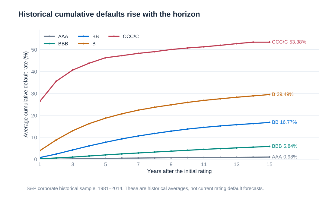
For example, the historical BBB rate is 0.20% at one year and 1.95% at five years, whereas the corresponding B rates are 3.88% and 18.70%. Cumulative default probability rises with the horizon, but annual increments need not be constant. An initially strong borrower has time to deteriorate; an initially weak cohort also changes composition as vulnerable firms default and survivors remain. Consequently, multiplying a one-year rate by the number of years is not generally a sound method of estimating a multi-year PD.
Let denote cumulative default probability, with default time and . The unconditional probability of default during year is . The conditional probability, given survival to the beginning of that year, is
For the BBB observations, the second-year unconditional increment is . The corresponding conditional probability is . These quantities are close for a low-risk cohort but differ materially when cumulative default rates become large. Under a constant annual conditional probability , survival through years is and cumulative PD is .
The historical timing graphic below has a different denominator: it tracks the timing of defaults among firms that ultimately defaulted in its 1981–2012 sample, grouped by initial rating. It illustrates how quickly eventual defaulters reached default. Its percentages must not be read as unconditional annual PDs for all firms initially assigned a rating or used interchangeably with the cumulative-rate table.
Internal scores, financial ratios and classification
An internal rating starts with quantitative and qualitative information about an obligor. A basic score may then be changed by warning signals, exceptional circumstances, support from a parent or guarantor, and a documented override. The resulting obligor grade should be distinguished from an assessment of a particular facility: collateral and seniority can materially change LGD without improving the borrower's ability to avoid default. A score is ordinal if it only ranks borrowers; it becomes a metric measure of risk only after calibration to a probability or expected-loss quantity.
A linear score has the form , where are borrower characteristics and are fitted coefficients. Profitability and leverage often move creditworthiness in opposite directions, but the score's sign convention must be specified. If higher means stronger credit, a profitability coefficient may be positive and a leverage coefficient negative. Combining these dimensions creates a boundary between classifications; it does not establish that the chosen ratios alone cause future default.
The following historical illustration uses an Altman-style modified score:
where is working capital divided by total assets, retained earnings divided by total assets, EBIT divided by total assets, and market value of equity divided by book liabilities. This is the particular specification used in the illustration, not a universal Altman formula: published Z-score variants differ in coefficients, equity definitions and the population for which they were developed. Mixing one variant's inputs with another variant's thresholds invalidates the interpretation.
| Input or result | BMW | Daimler |
|---|---|---|
| Working capital | −0.25 | 3.18 |
| Retained earnings | 20.42 | 19.36 |
| EBIT | −0.22 | 3.48 |
| Market value of equity | 19.28 | 25.46 |
| Sales (not used in this formula) | 51.42 | 87.49 |
| Total assets | 101.86 | 127.28 |
| Book liabilities | 79.70 | 96.67 |
| Calculated score Z | 4.13 | 4.37 |
| Illustrative score-mapped grade | B | B+ |
The displayed inputs produce for BMW and for Daimler. The B and B+ labels belong to this illustration's score mapping, not to a verified claim about either company's actual agency rating in 2008. The source's monetary scale is ambiguous, so the table preserves the common-scale inputs and explicitly treats them as ratio-building data rather than audited euro amounts. Sales are shown for completeness but do not enter this particular four-ratio formula. Rescaling all monetary inputs by the same factor leaves every ratio and the score unchanged.
Any classification cutoff creates two kinds of error: a borrower later defaults after being classified as acceptable, or a borrower that would repay is classified as unacceptable. These are sometimes called Type I and Type II errors, but naming conventions differ. Stating the event explicitly is safer. Lowering approval standards can increase lending and interest income while admitting more eventual defaults. Tightening standards reduces that exposure but rejects some profitable good borrowers. The appropriate cutoff depends on losses, margins, operating costs and constraints, not on classification accuracy alone.
Logistic models and retail information
A logistic model maps a linear index to a number between zero and one:
The log-odds satisfy . A positive coefficient raises PD when the associated variable increases, holding the others fixed; its effect on probability is nonlinear and depends on the initial PD. As a purely mathematical illustration, crosses 50% at . Here is a dimensionless illustrative stress index. These coefficients are not presented as an estimated or validated credit model, and they must not be used to approve a loan.
Retail credit assessment may use income and expenditure information supplied to the lender, assets and existing liabilities, employment stability, contractual loan features and observed payment behaviour. Account conduct can reveal persistent overdrafts, irregular inflows or missed payments. Credit registries can add information about obligations with other institutions and adverse payment events. No single variable substitutes for a documented assessment of repayment capacity, and a registry score is not the same thing as the lender's affordability calculation.
Historical lists of potential model inputs include demographic characteristics, residential location and behavioural proxies. Such availability does not make an attribute appropriate to use. Data relevance, accuracy, lawful processing, discriminatory effects and the possibility that apparently neutral variables proxy protected characteristics require separate assessment. Information collected for credit assessment also needs a defined retention policy and a way to correct errors; a historical example of a retention period is not a rule applying to every record today.
SCHUFA provides a useful example of a German credit-information system. Its records can include identifying information, credit and account relationships, inquiries and payment disruptions. Its new score introduced in March 2026 uses 12 criteria and a scale from 100 to 999. These criteria concern payment disruptions; the age of the oldest bank contract and oldest credit card; address tenure; the age of the youngest revolving facility; recent banking and non-banking inquiries or contracts; recent instalment loans and their longest remaining maturity; credit status; mortgages; and identity checks. SCHUFA states that it does not know a person's income, wealth, marital status or religion.
Current description: SCHUFA's twelve score criteria and information not held by SCHUFA. The score's introduction date and criteria replace older, inconsistent descriptions.
A December 2025 newspaper example concerning a credit-card provider change illustrates why consumers may question changes in a registry score even when their income has not changed. The case concerns a historical scoring environment and does not establish the effects of every card switch under the later model. The general analytical point is that a statistical score responds to the information and design of that model, whereas actual repayment capacity also depends on circumstances outside it.

Calibration, discrimination and validation
A model can rank borrowers well while producing inaccurate probabilities, or produce a reasonable portfolio average while ranking individuals poorly. Calibration asks whether predicted PDs agree with observed default frequencies over the relevant horizon. Discrimination asks whether eventual defaulters receive worse scores than survivors. Stability asks whether these properties persist across time, industries and borrower populations. Validation must examine all three rather than treating a single goodness-of-fit statistic as sufficient.
For corporate portfolios, quantitative financial ratios are supplemented by forecasts, management quality, competitive position and industry conditions. An accounting-based rating need not react immediately to market spreads; a market-implied model will respond faster but also incorporates risk premia and liquidity. A through-the-cycle system and a point-in-time system can legitimately behave differently. Calibration requires a default definition, a reference population, a horizon and representative data, including downturns where available. Regulatory IRB standards impose data-history and conservatism requirements. For corporate PD estimation, the historical observation period must cover at least five years; longer relevant available histories should be used. Five years of history are not the same as five borrower observations, and meeting a minimum period alone does not make a model reliable.
Data-history reference: Basel CRE36 minimum requirements for IRB models.
Consider two illustrative classifications of the same-sized portfolio of 100 loans with 20 eventual defaults. Classes are ordered from highest to lowest risk. In example A, default rates are 60%, 40%, 20% and 8%; example B changes the first two class sizes and default counts. Keeping the examples separate matters because their accuracy ratios are similar but not identical.
| Risk class | A: loans | A: defaults | A: default rate | B: loans | B: defaults | B: default rate |
|---|---|---|---|---|---|---|
| 1 (highest risk) | 10 | 6 | 60% | 5 | 4 | 80% |
| 2 | 10 | 4 | 40% | 15 | 6 | 40% |
| 3 | 30 | 6 | 20% | 30 | 6 | 20% |
| 4 (lowest risk) | 50 | 4 | 8% | 50 | 4 | 8% |
| Total | 100 | 20 | 20% | 100 | 20 | 20% |
A cumulative accuracy profile, or CAP, plots the proportion of all eventual defaults captured against the proportion of borrowers selected, starting with the riskiest scores. Random ranking follows the diagonal. Perfect ranking places all 20 defaults first, reaches 100% of defaults after 20% of borrowers, and is flat thereafter. The accuracy ratio is the area between the model curve and the random diagonal divided by the corresponding area for perfect ranking.
For example B, the CAP points are , , , and . Joining these points linearly, the area under the curve is 0.7025. The random area is 0.5 and the perfect area is 0.9, so
Example A gives an area of 0.7000 and an accuracy ratio of 50%. These figures measure ranking power for the constructed samples; they do not mean that the model predicts each default with 50% accuracy. A good validation also checks calibration by grade, uncertainty from small samples, overrides, data quality and out-of-sample performance. Perfect retrospective ranking can reflect overfitting rather than usable forecasting ability.
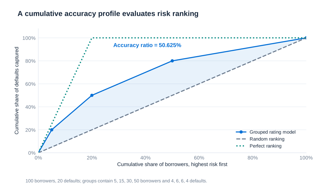
Credit deterioration, accounting losses and capital pressure
The financial crisis exposed weaknesses in securitisation ratings, internal-model incentives, counterparty assessment and reliance on apparently safe sovereign assets. Complex structures could concentrate systematic exposures while appearing diversified. Institutions could also postpone recognition of weak lending through repeated refinancing or restructuring that failed to restore sustainable repayment capacity. A new contractual maturity does not by itself cure an economic credit problem.
Policy responses included changes to trading-book and securitisation capital, stronger treatment of non-performing exposures, limits on internal-model variability, stress testing, and collateral or central-clearing requirements for eligible derivatives. These address different channels: a capital rule increases resilience to loss, a stress test studies adverse scenarios, and collateral reduces unsecured counterparty exposure. None makes underlying borrower defaults impossible. The historical term Basel 2.5 refers to an earlier set of trading-book reforms, whereas CRR3 implements later revisions in the EU.
Fair-value measurement also needs care. Level 1 uses quoted prices in active markets for identical assets or liabilities; Level 2 uses other observable inputs; Level 3 uses significant unobservable inputs. The hierarchy concerns valuation inputs, not a permanent classification of entire security types. A valuation adjustment may reflect counterparty credit risk (CVA), own credit risk (DVA), funding effects (FVA) or liquidity assumptions sometimes described as LVA. These labels do not justify mechanically adding overlapping discounts: the valuation method and applicable accounting rules must avoid double counting.
For the input hierarchy, see IFRS 13 Fair Value Measurement.
A broad credit shock can hit a bank through several routes simultaneously. New defaults and revised recoveries increase credit losses; deteriorating performing exposures can require greater expected-loss allowances; traded credit assets can fall in fair value; and higher PDs, LGDs or weaker ratings can increase RWA. Earnings and capital may therefore fall while the capital requirement rises. Attempts by many banks to reduce lending at the same time can amplify a downturn through a credit crunch.
A historical first-quarter 2020 Credit Suisse example makes these distinctions concrete. The original figures are in CHF millions, not euros, and the allowance treatment refers to US GAAP CECL rather than IFRS 9. Credit-loss provisions are not limited to losses on loans that have already defaulted. The following bridge keeps allowance movements and fair-value marks separate before reproducing the broader reported reserve-build measure.
| Component | Amount | Interpretation |
|---|---|---|
| Credit-loss provisions | 568 | Income-statement charge; includes expected losses |
| Net write-offs and other allowance movements | −55 | Other changes in the allowance |
| CECL adoption effect | 72 | Transition effect included in the allowance increase |
| Increase in credit-loss allowance | 585 | 568 − 55 + 72 |
| Leveraged-finance fair-value marks | 284 | Separate mark-to-market component |
| Asia-Pacific financing fair-value marks | 160 | Separate mark-to-market component |
| Total fair-value marks | 444 | 284 + 160 |
| Total reported reserve build | 1,029 | 585 + 444 |
| Of which: CECL-related component | 376 | 72 adoption + 304 additional build; already included above |
| Other component of reported reserve build | 653 | 1,029 − 376; not an additional charge |
The CHF 376 million CECL-related component consists of the CHF 72 million adoption effect and CHF 304 million of additional allowance build; it is part of the total, not a further amount to add to CHF 1,029 million. The remaining CHF 653 million completes that presentation. This example shows why a headline reserve-build number must be reconciled to its components before being interpreted as realised default losses or as a single accounting provision charge.
Portfolio loss, dependence and economic capital
A portfolio model combines individual exposure characteristics with the way defaults, migrations and recoveries co-move. Independent small exposures diversify more effectively than a few large exposures or many borrowers linked to the same sector, region or economic factor. Expected loss adds across borrowers regardless of dependence, but the tail of the total-loss distribution can change dramatically. A portfolio can therefore have the same EL as another and need much more capital to absorb adverse outcomes.
Write borrower loss as , where equals one after default and zero otherwise. Total loss is . Its variance includes both individual variances and pairwise covariance terms:
Independence removes the covariance terms, but it is a strong assumption. A recession can simultaneously increase default probabilities, reduce collateral prices and lengthen recovery procedures. This creates adverse dependence between default rates and LGDs, so a constant recovery assumption can understate severe losses. Shared counterparties, supply chains and funding sources can add concentration beyond broad sector labels.
In a one-factor Gaussian model, a latent asset return is , where the systematic factor and idiosyncratic shocks are independent standard normal variables. Borrower defaults if . Conditional on , its PD is . The parameter is an asset-factor correlation, not the default-indicator correlation itself.
For an infinitely granular homogeneous portfolio with constant LGD, the model's loss-rate quantile is
With PD 2%, LGD 45% and a 99.9% confidence level, increasing from 0.05 to 0.25 raises the quantile from approximately 3.6465% to 12.5323% of total exposure, although EL remains 0.9%. This is a different, asymptotic model from the earlier finite portfolio of 100 independent loans. The graph compares exceedance probabilities on a logarithmic vertical scale: a 0.1% tail probability marks the 99.9% quantile.
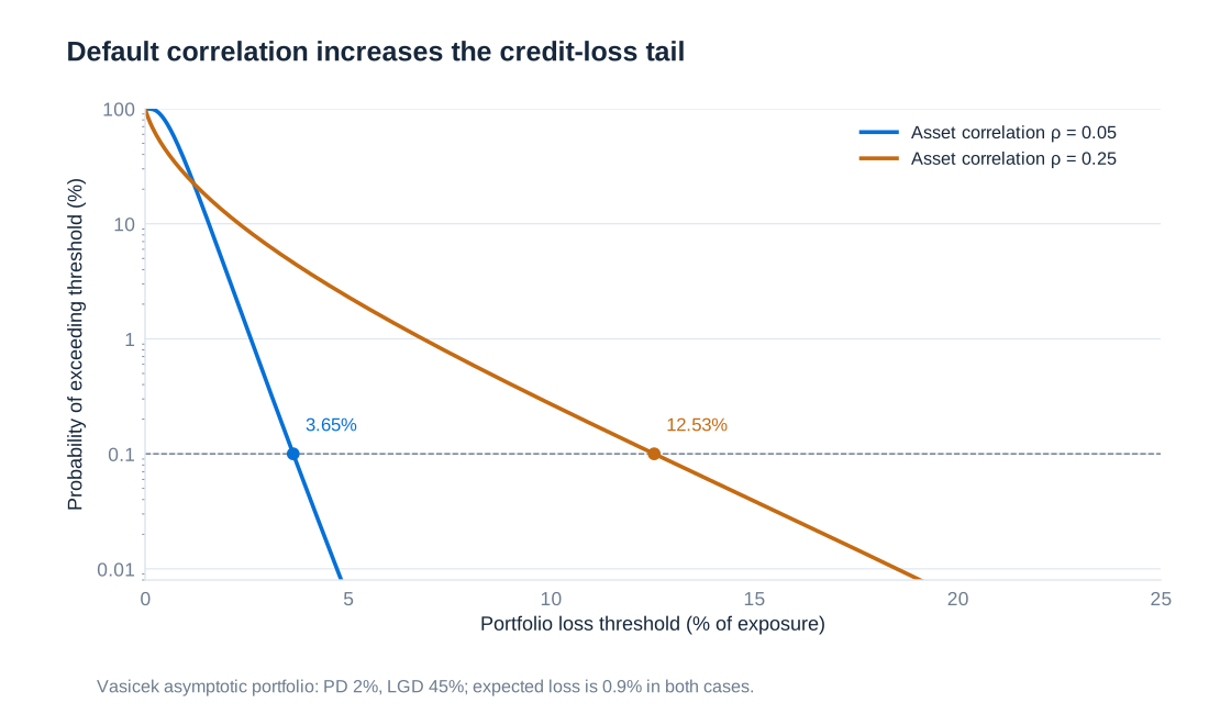
Monte Carlo simulation implements more elaborate versions by repeatedly drawing common factors and borrower outcomes, applying exposures and recoveries, and collecting total losses or changes in value. The average simulated loss estimates EL; a selected quantile estimates VaR; their difference measures quantile-based economic capital under the stated convention. A 99.98% confidence level is one possible internal choice, not a universal requirement. A higher confidence level also makes tail estimation more demanding, especially when extreme losses are rare.
CreditMetrics and migration risk
A default-only model ignores losses from worsening credit quality before default. CreditMetrics-style models instead allow each borrower to migrate among rating states over a horizon. Each non-default state receives a horizon value obtained by discounting the remaining cash flows using rates appropriate to that state. The default state receives a recovery value. The resulting distribution includes gains from upgrades, losses from downgrades and losses from default.
A transition matrix states the probabilities of moving from each initial rating to each ending rating. The historical matrix below is an adjusted example from the CreditMetrics technical document, based on S&P transition information and adjusted to match long-term probabilities. It is not a current matrix or an unadjusted Moody's estimate. Values are percentages; the absorbing default row is added explicitly as 100%, not 1%. Small deviations of a row sum from 100% reflect the displayed rounding.
| Initial rating | AAA | AA | A | BBB | BB | B | CCC | Default |
|---|---|---|---|---|---|---|---|---|
| AAA | 87.74 | 10.93 | 0.45 | 0.63 | 0.12 | 0.10 | 0.02 | 0.02 |
| AA | 0.84 | 88.23 | 7.47 | 2.16 | 1.11 | 0.13 | 0.05 | 0.02 |
| A | 0.27 | 1.59 | 89.05 | 7.40 | 1.48 | 0.13 | 0.06 | 0.03 |
| BBB | 1.84 | 1.89 | 5.00 | 84.21 | 6.51 | 0.32 | 0.16 | 0.07 |
| BB | 0.08 | 2.91 | 3.29 | 5.53 | 74.68 | 8.05 | 4.14 | 1.32 |
| B | 0.21 | 0.36 | 9.25 | 8.29 | 2.31 | 63.89 | 10.13 | 5.58 |
| CCC | 0.06 | 0.25 | 1.85 | 2.06 | 12.34 | 24.86 | 39.97 | 18.60 |
| Default | 0.00 | 0.00 | 0.00 | 0.00 | 0.00 | 0.00 | 0.00 | 100.00 |
Each row conditions on the initial rating, so reading the table by columns answers a different question. For example, the BBB row assigns 84.21% to remaining BBB and 0.07% to default over the model horizon. The table cannot alone predict the starting composition of a portfolio or the fraction of defaults originating in BBB. When it is used numerically, minor rounding discrepancies should be handled transparently, for example by normalising the displayed row within its rounding tolerance.
If the transition mechanism is assumed stationary and Markovian, a multi-period transition matrix is a power of the one-period matrix: . This assumption says that the current rating contains the relevant migration information and the probabilities remain stable. Rating history, the business cycle and changing market conditions can violate it. Multiplying matrices is therefore a modelling operation, not a factual statement that historical transitions will repeat.
Portfolio implementation needs dependence between migrations as well as individual transition probabilities. CreditMetrics uses a latent-variable framework in which rating thresholds and asset-return correlations generate joint states; equity-return information may be used as a proxy when suitable. Each simulated joint outcome is then revalued. Recovery assumptions, concentration and the sensitivity of state values to interest rates and credit spreads can all affect the tail. Model comparison should keep the horizon, valuation basis and confidence level consistent.
Historical matrix and methodology: CreditMetrics Technical Document, Table 6.11. The example is preserved as a historical model illustration.
Managing the exposure and its residual risks
Credit-risk management begins before a loan is made: underwriting, exposure limits, pricing, covenant design and sector diversification determine the initial risk. Monitoring then tracks financial deterioration, missed payments and other warning signals. Collateral can lower loss severity if it is legally enforceable and retains value in the default scenario. A guarantee transfers exposure to the guarantor and must be assessed in light of that party's own capacity and possible correlation with the borrower.
Contractual tools can include material-adverse-change clauses, review or cancellation rights for uncommitted facilities, and shorter refinancing periods. Their practical effect depends on the agreement and applicable law. They may limit future lending but do not automatically recover money already advanced. A withdrawal of liquidity can also worsen the borrower's position, which makes early monitoring and orderly restructuring more useful than a purely mechanical response to a score.
Netting reduces exposure only when the relevant arrangements are legally effective and cover the obligations in question. Derivative protection introduces counterparty risk; a securitisation can leave retained tranches, servicing obligations or contingent liquidity facilities. The historical IKB/Rhineland experience illustrates why an apparently separate vehicle can return risk to a sponsoring bank through support commitments or funding stress. An off-balance-sheet label is therefore not enough to establish economic risk transfer.
CDS and asset-backed structures provide additional tools for altering the distribution of credit exposure. Their value lies in the precise contractual transfer they achieve, not in removing credit risk from the financial system. The next chapter follows their cash flows, identifies who bears each loss, and separates credit protection from funding, liquidity and counterparty effects.
8. Credit Default Swaps and Asset-Backed Securities
Credit risk can be transferred through a derivative contract or through the sale and financing of assets. A credit default swap separates a specified credit exposure from ownership of the underlying bond or loan. A securitisation places assets or their risks into a structure that distributes cash flows and losses among investors. Both can change who bears credit losses, but neither removes those losses from the economy. Understanding the contracts requires following the cash flows, the loss allocation and the obligations that remain after the transaction.
The credit default swap contract
A credit default swap, or CDS, is a contract under which a protection buyer pays a premium to a protection seller in exchange for a payment if a specified credit event affects a reference entity or obligation. The economic analogy with insurance is useful: the buyer pays for protection and ordinarily receives no credit-event payment when the covered event does not occur. A CDS is nevertheless a derivative with its own contractual and legal framework; it should not be assumed to have every feature of an ordinary insurance policy.
The contract identifies the reference entity, eligible obligations, notional amount, currency, maturity, premium terms, credit-event definitions and settlement method. A credit event can include failure to pay, bankruptcy or qualifying restructuring, depending on the agreed terms. A fall in the bond price alone does not necessarily trigger settlement. The reference entity whose credit is being transferred is distinct from the protection seller, whose ability to perform creates counterparty risk.
The notional amount is a reference for calculating premiums and settlement. It is not generally a sum that the buyer lends to the seller at inception. The premium rate is quoted annually, often in basis points: one basis point equals 0.01 percentage points or 0.0001 in decimal form. Payment frequency and the day-count convention determine the amount paid on each date. A five-year semiannual example is convenient for learning, but frequency and market conventions must be read from the actual contract.
A five-year protection example
Consider a CDS referencing IBM, with USD 100 million notional, a five-year maturity and a premium of 90 basis points per year. This is a numerical illustration, not a current IBM market quotation. Since 90 basis points equals 0.90%, the annual premium is dollars. Under an exact half-year payment assumption, each semiannual premium is USD 450,000.
| Quantity | Value | Meaning |
|---|---|---|
| Notional | USD 100 million | Reference amount for premiums and protection |
| Annual premium rate | 90 bps = 0.90% = 0.009 | Annualised contractual rate |
| Annual premium | USD 900,000 | 100,000,000 × 0.009 |
| Semiannual premium | USD 450,000 | 900,000 × 0.5 |
| Number of payments without a credit event | 10 | Five years with two payments per year |
| Undiscounted total without a credit event | USD 4.5 million | 10 × 450,000; ignores upfront amounts and fees |
If no credit event occurs before maturity, the buyer pays the scheduled premiums and receives no default settlement. The premiums are the price of the protection already provided; they are not returned because the reference entity survives. If a qualifying event occurs earlier, future scheduled premiums generally stop, while premium accrued up to the event remains payable according to the contract. A default between payment dates therefore cannot be analysed simply by ignoring the incomplete period.
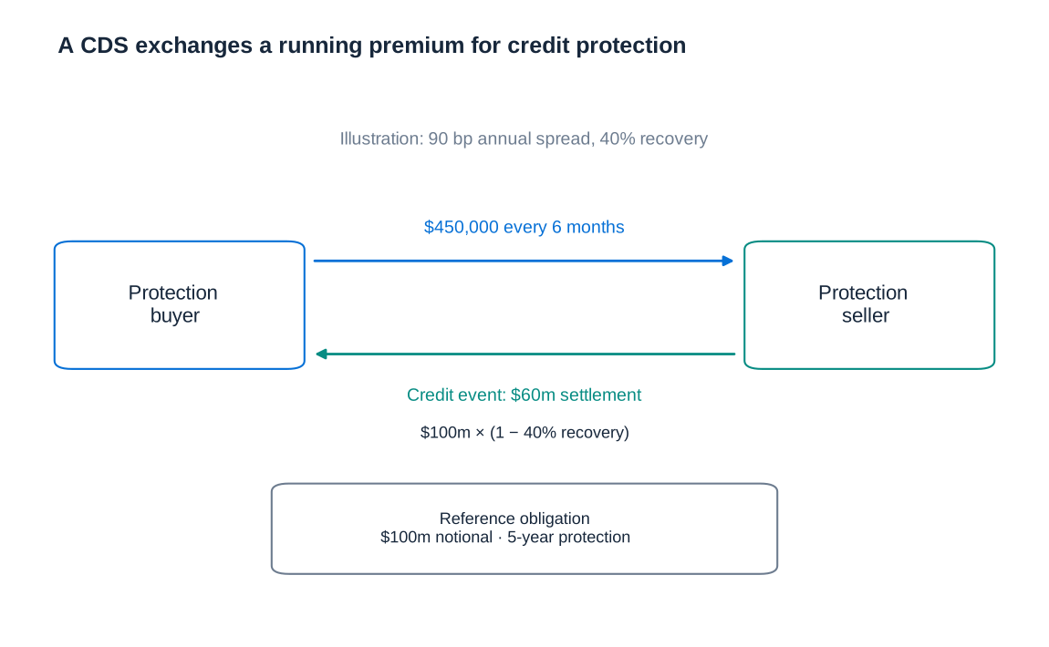
Physical and cash settlement
Under physical settlement, the protection buyer delivers an eligible defaulted obligation and receives the agreed par amount from the protection seller. In the USD 100 million example, a buyer delivering eligible bonds with USD 100 million face value receives USD 100 million. The delivered bonds have a residual value, so the seller's economic loss is less than the gross cash payment whenever recovery is positive. Eligibility, deliverable-obligation provisions and settlement mechanics are material contractual details.
Under cash settlement, the seller pays the difference between the contractual reference amount and the value established for the defaulted obligation. With notional and recovery fraction , the simplified protection payment is . If recovery is 40%, cash settlement on USD 100 million is USD 60 million. In an equivalent physical settlement, the buyer transfers bonds worth USD 40 million and receives USD 100 million, again generating a net economic protection amount of USD 60 million before premiums and other costs.
The protection buyer, not the seller, is entitled to the default payment. The payment compensates for the specified reference-credit loss; it does not necessarily reimburse every loss on a separately held asset. Differences in maturity, currency, seniority, deliverable obligations or contractual credit-event definitions can leave basis risk. A lender hedging a loan must therefore check that the CDS protection actually responds to the scenarios that threaten that loan.
The premium leg, protection leg and market value
At inception, an idealised par CDS with no upfront payment has equal present values for the premium and protection legs. Let be the risk-neutral probability that the reference entity survives to time , the discount factor, a premium date, its year fraction, the annual premium rate and the notional. With deterministic recovery fraction , a useful representation is
The term is the expected discounted premium-accrual fraction paid when default occurs between scheduled dates. Both expressions are in currency units. The protection leg integrates the probability of first default at each time; it must not count the same entity as defaulting repeatedly. The par spread solves . Real valuation also needs the exact contract, discounting conventions and relevant counterparty or collateral treatment.
In a continuous-premium model with constant risk-neutral default intensity and constant recovery, the simple relation is . It provides intuition: a larger default intensity or a larger loss severity requires a larger premium. At 90 basis points and 60% LGD, the implied intensity is , or 1.5% per year. Under these assumptions, five-year risk-neutral cumulative PD is . The annual CDS spread is therefore neither the annual PD nor the five-year PD.
This probability is risk-neutral because it is inferred from prices. It is not an unbiased forecast of real-world defaults. Market spreads can reflect default-risk compensation and liquidity as well as expected loss. The simplified intensity relation also abstracts from term structures, discrete premiums and several contractual effects. It should be used as a transparent approximation, not as an exact recovery of physical PD from an observed quotation.
After inception, a CDS can acquire positive or negative market value. If the market spread rises while the buyer continues to pay an older, lower contractual rate, that protection becomes valuable to the buyer. Approximately, buyer value is , where is the risky premium annuity, expressed in years and incorporating survival and discounting. The seller has the opposite value before counterparty and other asymmetries. If spreads fall, the buyer's position usually loses value. This allows a CDS position to generate gains or losses before any default occurs.
Some market contracts use standardised running coupons with an upfront amount to reconcile that coupon with the current market spread. “No initial exchange of notional” therefore does not mean “no initial cash requirement”: an upfront amount, initial margin and transaction costs may all arise.
For the distinction between a standard coupon, an upfront amount and market value, see ISDA's explanation of CDS collateral and pricing conventions.
Hedging, diversification and taking credit exposure
A bank can buy protection to reduce exposure to a borrower or sector while retaining the underlying customer relationship. It can also sell protection to take credit exposure in a sector where it has little direct lending. This can diversify some risks, but diversification should be evaluated against the bank's entire balance sheet: exposures that appear unrelated in ordinary conditions may become correlated during a downturn.
A non-bank investor selling protection receives premium income in exchange for bearing a contingent credit loss. This resembles taking a funded credit position in its direction of exposure, but the seller must be able to meet margin calls and a potentially large settlement payment. The premium is compensation for risk, not a guaranteed yield free of a corresponding obligation.
Buying protection without owning the reference bond creates a position that can benefit from deterioration or default. Economically this resembles a short-credit position, although its funding, contractual and legal characteristics differ from short-selling a bond. A profitable directional prediction still can be undermined by counterparty default, changing liquidity, transaction costs or a mismatch between the expected event and the contract's actual trigger.
Counterparty exposure before and after a credit event
CDS transfer reference-credit risk while creating exposure to the contractual counterparty. If the protection seller defaults after a covered credit event but before paying, the buyer may be left with an unsecured claim for the settlement amount, reduced by available collateral and enforceable netting. The reference entity and protection seller can fail in the same stressed environment. A hedge that depends on a weak seller may consequently fail just when it is most valuable.
Before a reference-credit event, the buyer's exposure is the positive replacement value of the contract, not automatically its full notional. Suppose market protection has become more expensive than the contractual premium. If the seller fails, replacing that low-premium contract requires paying the higher current price. The resulting loss is associated with the present value of the premium difference, subject to close-out terms, recovery, collateral and netting.
The seller can also have counterparty exposure. If market spreads have fallen below the premium it is entitled to receive, its existing contract is valuable. A default by the protection buyer can force the seller to replace it with a contract paying a lower premium. Losing future gross premiums is not by itself the correct exposure measure because the seller also ceases to bear the original future protection obligation; valuation concerns the net replacement position.
Wrong-way risk arises when counterparty creditworthiness deteriorates as exposure to that counterparty increases. A protection seller heavily exposed to the same sector as the reference entity is an obvious example. Correlated defaults can defeat a simple calculation that multiplies an independently estimated counterparty PD by an average exposure. Effective risk management therefore examines joint stress scenarios and the strength of collateral and close-out arrangements.
Collateral, margin and central clearing
Variation margin addresses changes in the current market value of a derivative. When the contract becomes more valuable to one party, collateral is transferred by the other under the relevant agreement. Initial margin addresses potential changes in exposure over the period needed to close out or replace positions after a default. Both sides can have collateral obligations. Margin reduces unsecured exposure but introduces liquidity needs: an institution may have to deliver cash or eligible securities quickly even though the reference entity has not defaulted.
Collateral protection depends on timely valuation, settlement, enforceability, segregation where required, eligible collateral and haircuts. A haircut reduces the recognised value of collateral to allow for adverse movements or liquidation costs. Collateral closely linked to the counterparty's financial condition can create wrong-way risk. Disputes, market jumps and delays mean that collateralisation does not mechanically eliminate every possible loss.
Central clearing replaces a bilateral relationship with cleared obligations involving a central counterparty, or CCP. The CCP manages exposures through margin, default-management procedures and financial resources. Central clearing is distinct from exchange trading: an OTC contract can be centrally cleared. A CCP is not risk-free and should not be described as possessing a fictitious “AAAA” rating. Clearing concentrates important risk-management functions and creates its own operational, liquidity and default-management requirements.
In the EU, EMIR provides clearing obligations for specified classes of OTC derivatives and relevant categories of counterparties, together with risk-mitigation requirements for non-cleared contracts. Applicability depends on the instrument class, counterparty status, thresholds and exemptions; it is incorrect to say that every CDS must be traded on an exchange or centrally cleared. Exact transaction requirements should be checked against the applicable rules and registers.
Regulatory reference: ESMA on clearing and non-cleared risk mitigation under EMIR.
True-sale securitisation and the special-purpose vehicle
An asset-backed security, or ABS, is financed by cash flows from a defined asset pool. Typical pools contain loans, mortgages, leases or trade and consumer receivables. In a traditional true-sale structure, an originator sells or assigns the assets to a special-purpose vehicle, or SPV. The vehicle raises funding by issuing securities to investors and uses the proceeds to pay for the assets. The borrowers' payments then support the securities, after contractual costs and other senior claims.
The SPV separates the transaction's assets and obligations from the originator's ordinary business, but the legal effectiveness of that separation matters. Bankruptcy remoteness does not mean that the underlying borrowers cannot default. Investors also depend on servicing, collection accounts, documentation and the availability of replacement providers if a service counterparty fails. A diagram showing an asset transfer is the beginning of analysis, not proof that every risk has left the originator.
The originator often continues as servicer, collecting payments and managing the borrower relationship for a fee. Borrowers may continue making payments through the same channels, but legal transfer, notification, data-processing and contractual requirements can still matter. Securitisation should not be described as necessarily changing nothing for every borrower. The operational process and the ownership of the credit exposure are separate questions.
Pass-through securities and cash-flow timing
A pass-through structure distributes the available pool cash flows to investors according to their proportional interests, after fees and other specified deductions. It is simpler than a structure with several different priorities, but it still transmits the risks in those cash flows. Defaults reduce collections, recoveries can be delayed, and early repayments change the timing of principal returned to investors.
Prepayment risk is especially important for assets whose borrowers can repay early. If borrowers refinance when interest rates fall, investors may receive principal back when reinvestment yields are lower. Conversely, slower-than-expected repayment can extend the investment's duration. Credit loss, prepayment and extension risk are distinct, and a high-quality borrower pool can still produce uncertain cash-flow timing. The security's expected maturity need not equal its legal final maturity.
Tranching, subordination and the waterfall
Tranching divides a pool into securities with different priorities. Senior claims are paid before junior or mezzanine claims under the specified payment waterfall, and the equity or first-loss piece receives the residual. Loss allocation ordinarily runs in the opposite direction: equity absorbs losses first, then mezzanine claims, then senior claims. Actual structures can have separate interest and principal waterfalls, reserve accounts and performance triggers, so their detailed documents control the sequence.
Consider a simplified pool with initial principal 100 monetary units. Equity covers the first 20 units of loss, mezzanine the next 20, and senior notes the remaining 60. The mezzanine band can be divided further into a lower band covering losses from 20 to 30 and an upper band covering losses from 30 to 40. Historical illustrations sometimes label these bands BB and BBB and the senior notes AAA. Such labels are illustrative outcomes of a rating process, not a consequence guaranteed solely by drawing the boundaries.
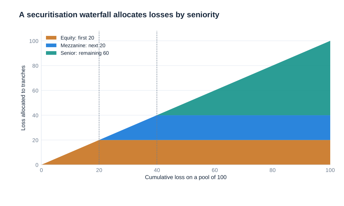
For a tranche attaching at and detaching at , both measured in pool currency units, and cumulative pool loss , the simplified principal loss is
Dividing this amount by the tranche's original principal gives its loss fraction. The formula assumes a static pool, no changing credit enhancement and direct sequential allocation of realised principal losses. It explains subordination transparently without claiming to reproduce every feature of a live securitisation.
| Pool loss | Equity loss: 0–20 band | Mezzanine loss: 20–40 band | Senior loss: 40–100 band | Senior loss fraction |
|---|---|---|---|---|
| 0 | 0 | 0 | 0 | 0% |
| 5 | 5 | 0 | 0 | 0% |
| 25 | 20 | 5 | 0 | 0% |
| 45 | 20 | 20 | 5 | 8.33% |
| 80 | 20 | 20 | 40 | 66.67% |
| 100 | 20 | 20 | 60 | 100% |
A pool loss of 25 therefore destroys the equity piece and one quarter of the 20-unit mezzanine tranche while leaving senior principal intact in this model. A pool loss of 45 reaches the senior notes and removes 5 of their 60 units, or 8.33%. A tranche can be protected against frequent small losses while remaining exposed to infrequent large losses. Ratings, expected losses and tail-loss severity consequently describe different aspects of its risk.
Funding, capital treatment and retained interests
Securitisation can provide funding, diversify funding sources, transfer selected credit exposures and change the maturity or risk profile of the originator's balance sheet. Cash proceeds may be used to repay existing debt, which can reduce leverage under the relevant measurement. However, issuing securities through an SPV does not automatically increase profitability or return on equity. Fees, funding costs, transaction expenses, retained risk and the use of the proceeds all influence the result.
Legal true sale, accounting derecognition, consolidation and regulatory capital relief are separate assessments. An asset transfer does not necessarily remove the assets from consolidated financial statements, and accounting derecognition alone does not establish sufficient prudential risk transfer. Regulatory capital relief depends on the applicable significant-risk-transfer requirements and the treatment of retained or otherwise exposed positions. A claim that RWA must fall by the full amount of the transferred assets would ignore those conditions.
The originator may retain equity, mezzanine or a proportional share of the transaction. Retaining a first-loss tranche can preserve substantial credit exposure even when most of the face value is sold. It is also incorrect to assume that only senior notes can be placed with investors: placement depends on price, structure, market conditions and investor mandates. Liquidity facilities, guarantees or other support can create additional exposures outside the retained securities.
EU rules generally require an originator, sponsor or original lender to retain at least 5% of a material net economic interest, subject to the regulation's specified methods and exceptions. Retention can take different forms, including a vertical share of tranches or an eligible first-loss position; it is not a universal instruction to keep the entire equity tranche. The requirement is intended to maintain an economic stake and does not establish that the retained party bears every possible loss.
References: EBA on significant risk transfer; Article 6 of the EU Securitisation Regulation.
Resecuritisation and the limits of ratings
A collateralised debt obligation, or CDO, can hold debt claims that include tranches from other securitisations. Repackaging mezzanine ABS into a new structure creates another layer of senior, junior and equity claims. It reallocates the losses on the purchased tranches; it does not turn the original borrowers into safer borrowers. The outer structure's risk depends on the attachment points and loss distributions of the inner structures as well as on their dependence.
Correlation is especially important. Under a benign model, losses in different pools may rarely occur together, so a new senior tranche appears well protected. A common housing or funding shock can make many mezzanine tranches lose value at the same time, exhausting that protection. Two layers of modelling can magnify errors in default probabilities, recoveries, dependence and asset selection. Complexity also makes it harder for investors to identify overlapping underlying exposures.
A high rating therefore cannot replace analysis of the pool, waterfall, model assumptions and stress scenarios. A tranche's market liquidity can deteriorate even without realised principal loss, and a mark-to-market loss can be much larger than a near-term expected default loss. The credit-crisis experience with structured products illustrates the importance of separating a contractual priority from an unconditional guarantee of safety.
Comparing funded securities and CDS positions
Buying a credit-sensitive ABS and selling protection both take exposure to adverse credit outcomes, while buying protection takes the opposite direction. Their full economics are different. The ABS buyer ordinarily pays a purchase price and receives the security's cash flows. A CDS seller receives premiums but assumes contingent settlement and collateral obligations. Funding costs, interest-rate exposure, liquidity, counterparty risk and contractual basis can make the two positions behave differently even when their reference credit is closely related.
| Position | Main cash commitment | Effect of worsening reference credit | Additional risks to assess |
|---|---|---|---|
| Long ABS | Purchase price, usually funded at inception | Potential price decline and allocated credit losses | Funding, liquidity, prepayment, servicing and structure |
| Sell CDS protection | Margin or upfront amounts where applicable; contingent default payment | Usually a market-value loss and greater potential settlement exposure | Counterparty exposure, margin liquidity and contract basis |
| Buy CDS protection | Premiums and applicable upfront or margin amounts | Usually a market-value gain; payment after a qualifying event | Seller default, imperfect hedge and settlement terms |
Accounting also depends on classification rules, not an unrestricted choice between reporting gains and hiding losses. Derivatives are generally measured at fair value through profit or loss unless qualifying hedge-accounting treatment changes how effects are presented. A debt security's measurement depends on the relevant business-model and contractual-cash-flow tests, which can lead to amortised cost, fair value through other comprehensive income or fair value through profit or loss. A structured instrument does not automatically qualify for amortised cost merely because the investor plans to hold it.
Accounting reference: IFRS 9 Financial Instruments.
The appropriate comparison starts with a common horizon and scenario: identify who pays, who receives, what event triggers each obligation, how losses are allocated, and what collateral or funding is needed along the way. This makes the transferred credit exposure visible while preserving the distinct risks created by the chosen instrument.
9. Earnings at Risk and Cash Flow at Risk
Three different objects of risk management
A financial position has a market value, produces accounting results and generates cash payments. These three descriptions are related, but they are not interchangeable. A bond can lose market value without changing its contractual coupon; a derivative can generate an immediate collateral payment while the benefit of the exposure it hedges will arrive years later. A useful risk analysis therefore specifies what must remain stable, for whom, and over what horizon.
Value at Risk concerns a distribution of economic or market-value losses. Earnings at Risk concerns a distribution of reported earnings, after applying the relevant recognition and measurement rules. Cash Flow at Risk concerns a distribution of cash receipts, payments or their net amount. Each requires a horizon, a confidence level and a precise boundary: consolidated earnings differ from one subsidiary’s earnings, and cash available in one currency or legal entity may not be available elsewhere.
Let denote earnings over horizon , net cash flow over that horizon, and the lower quantile of a random variable . One useful shortfall convention, adopted here, measures the distance from specified benchmarks and . At confidence level , define:
The benchmarks might be expected results or an approved budget; the choice must be disclosed. These measures are currency amounts, not probabilities. An EaR of €6 million does not mean that earnings will be negative by €6 million: it means that the selected lower-tail result is €6 million below the stated benchmark. Some organisations instead report the lower-tail earnings or cash-flow level itself. Reporting both the level and the shortfall prevents this terminology from obscuring the result.
Objectives, earnings expectations and managerial incentives
Different decision makers reasonably emphasise different outcomes. A bank manager may prioritise stable reported profits, a fund manager the value available to investors who redeem, and a household predictable mortgage instalments. A pension investor with known nominal payments may accept fluctuations in asset prices to secure the required future receipts. The correct objective depends on liabilities and withdrawal needs, not solely on the instrument’s standalone volatility.
The importance attached to recurring earnings is visible in public discussions of bank strategy. Morgan Stanley’s emphasis on more stable revenues in January 2023 illustrates the attraction of predictable business income. Debates about Josef Ackermann’s 25% return target at Deutsche Bank illustrate a different concern: a high return target can encourage leverage or risk taking if its risk cost is ignored. Stable reported earnings and a high reported return are not sufficient descriptions of a sound business model.
Market reactions also depend on expectations beyond the current earnings number. A company may beat analysts’ estimates while its share price falls because future guidance disappoints, discount rates rise or the result was already anticipated. Commentary on the second quarter of 2023 described precisely this combination. It does not establish that positive surprises are generally unwelcome. The quality, persistence and information content of earnings matter alongside their level.
Burgstahler and Eames (2006) examine how managers avoid negative earnings surprises. Their evidence links small non-negative surprises both to management of reported earnings and to management of analysts’ expectations, with roles for operating cash flows and discretionary accruals. For risk management, this raises a governance problem: an incentive to achieve a reported target can favour accounting outcomes over economic resilience. An instrument that smooths one reported number may increase financing needs elsewhere.
Choices can therefore involve genuine trade-offs. If strategy A has lower market-value risk but higher cash-flow risk than strategy B, neither dominates without information about the investor’s constraints. If A reduces all relevant risks for the same expected return and cost, B is harder to justify. A practical decision compares the full set of outcomes, including transaction costs, liquidity needs and the consequences of the adverse scenarios.
How accounting translates economic changes into earnings
Accounting determines when an economic change reaches profit or loss. Under IFRS 9, the classification of a debt financial asset depends principally on its business model and the characteristics of its contractual cash flows. The SPPI test asks whether those cash flows are solely payments of principal and interest on the principal outstanding. A prudential label such as “banking book” does not by itself establish the accounting category.
| Business model | Contractual cash-flow condition | Usual measurement category |
|---|---|---|
| Hold assets to collect contractual cash flows | SPPI condition satisfied | Amortised cost |
| Collect contractual cash flows and sell assets | SPPI condition satisfied | Fair value through other comprehensive income (FVOCI) |
| Other business models, or a failed SPPI condition | The preceding combinations do not apply | Fair value through profit or loss (FVTPL) |
The fair-value option can also be relevant when its conditions are met, including elimination or significant reduction of an accounting mismatch. Equity investments require separate classification considerations. The table is therefore a framework for ordinary debt assets, not a universal decision rule for every financial instrument.
Amortised cost does not mean that the balance-sheet amount remains permanently equal to purchase price. Effective-interest accruals, amortisation of premiums or discounts, repayments and expected credit losses can change the amount and the earnings recognised. What is generally absent is immediate recognition in profit or loss of every market-price movement caused solely by changes in market yields. For an FVTPL instrument, those valuation changes normally affect current earnings.
Other comprehensive income, or OCI, is outside the current profit-or-loss subtotal but remains part of comprehensive income and equity. A valuation movement reported in OCI has not disappeared economically. It can still affect capital, contractual constraints or the amount obtainable on sale. Risk managers must distinguish a stable profit-or-loss number from a stable balance sheet and from stable cash.
What hedge accounting changes
A derivative remains measured at fair value even when it participates in a qualifying hedge-accounting relationship. Hedge accounting changes the recognition of gains and losses to represent that relationship more faithfully. It requires an eligible relationship, documentation and satisfaction of the applicable effectiveness requirements; simply calling a transaction a hedge is insufficient.
The three main relationships have different accounting mechanics. In a fair-value hedge, changes in the hedging instrument and changes in the hedged item attributable to the designated risk generally enter profit or loss together. In a cash-flow hedge, the effective portion is initially recognised in OCI and is subsequently reclassified or incorporated into an asset’s carrying amount when the relevant rules require; ineffectiveness generally affects profit or loss. A hedge of a net investment in a foreign operation has an OCI treatment for its effective component associated with foreign-currency translation.
These distinctions explain why the statement “hedge losses go to OCI” is too broad. The accounting outcome depends on the designation and the underlying exposure. Moreover, no recognition rule cancels a derivative’s contractual settlement or collateral obligation. A hedge can improve the matching of reported earnings and still require substantial cash before the hedged transaction generates receipts.
Accounting sources: IFRS Foundation, IFRS 9 Financial Instruments, and the issued standard. Research reference: David Burgstahler and Michael Eames (2006), Management of Earnings and Analysts’ Forecasts to Achieve Zero and Small Positive Earnings Surprises.
One bond exposure, two financing and settlement patterns
Consider a hypothetical €100 long exposure to a very long-term bond with modified duration of 30 years. The exposure can be obtained by purchasing the bond or by taking an appropriately sized long position in a bond futures contract. Ignore basis changes and other differences initially. If the market yield rises by one percentage point, the first-order duration approximation is:
Here is the initial bond value, modified duration and the yield change expressed as a decimal. The 30% fall is an approximation; for such a large duration and yield shock, convexity can materially change the exact answer. This is a stress scenario, not a statistical VaR estimate unless a probability model and confidence level are supplied.
| Position and measurement | Economic value | Current earnings | Cash consequences after establishment |
|---|---|---|---|
| Purchased bond at amortised cost | Approximately €30 lower | No automatic €30 yield-driven fair-value loss; interest and impairment rules still apply | Contractual coupons continue if paid; a cash-funded holding has no futures variation margin |
| Purchased bond at FVTPL | Approximately €30 lower | Approximately €30 valuation loss in this simplified scenario | The valuation loss alone is not a cash payment; sale or secured financing can introduce cash effects |
| Long bond futures, without qualifying hedge accounting | Approximately €30 adverse change for matched exposure | Futures losses affect profit or loss | Variation margin produces cash payments as prices fall |
| Long bond futures in a qualifying hedge | The economic loss on the futures remains | Recognition depends on the designated hedge relationship | Collateral and settlement obligations remain payable |
The purchased bond requires the purchase price at inception. A futures position generally requires initial margin rather than payment of the full underlying value, but this smaller initial cash commitment is followed by potentially large variation-margin payments. Locating the futures in a particular management book does not remove these calls. If the purchased bond itself is financed through short-term borrowing or repo, its funding and collateral risks must also be added.
Thus similar interest-rate sensitivity can coexist with different EaR and CFaR. A statement that the directly purchased bond has “zero cash-flow risk” is defensible only within the narrow assumption of fixed contractual payments, no default, no optionality and no refinancing need. It is not a description of the investor’s entire balance sheet.
The perpetuity: stable income and unstable wealth
Suppose a 60-year-old retiree, Mr Rich, invests €10 million and wants a constant nominal income for an uncertain remaining lifetime. Assume a flat annual yield of 1% and an ideal default-free, non-callable perpetuity. A perpetuity pays the same amount at the end of every year forever. Its value is:
The yield is annual and expressed as a decimal; is euros per year and euros. Under these assumptions, the retiree receives €100,000 each year regardless of subsequent market yields. The investment meets the objective of constant nominal receipts without requiring a known date of death. It does not preserve purchasing power if prices rise, and real securities can introduce credit, call, tax and liquidity risks that the idealisation excludes.
| Market yield | Market value | Annual contractual income | Change from the initial €10 million value |
|---|---|---|---|
| 1% | €10,000,000 | €100,000 | €0 |
| 2% | €5,000,000 | €100,000 | −€5,000,000 |
| 5% | €2,000,000 | €100,000 | −€8,000,000 |
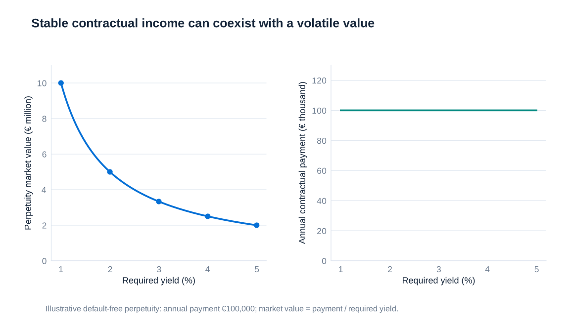
If the daughter inherits the security and immediately sells it after yields have risen to 5%, she receives €2 million. The same security is attractive to the father’s nominal-income objective and risky for the daughter’s eventual sale proceeds. The decline in market value reflects the lower attractiveness of the fixed coupon relative to newly available yields; it does not require any reduction in the promised coupon. A rise from 1% to 2% already halves the price, illustrating why percentage-point changes must be interpreted relative to the starting yield.
Fixed coupons, floating rates and the funding side
A floating-rate note resets its coupon periodically, for example every six months. A stylised coupon for period is , where is principal, the annual reference rate fixed for that period, the contractual annual spread and the year fraction. If the discount spread matches the contractual spread and credit and other conditions are unchanged, its ex-coupon value is approximately par at a reset date. Between resets, and when credit spreads change, its price can move.
The floating-rate investor therefore exchanges relatively stable interest-rate-related market value for variable future income. A fixed-rate investor makes the opposite exchange. A mortgage borrower who must meet instalments from a stable salary may value fixed nominal payments; a borrower expecting an early repayment may instead care about market-value changes and contractual termination charges. Neither preference is universal, and inflation changes the meaning of a “stable” nominal payment.
The same asset can also produce different earnings risk depending on the liabilities financing it. Suppose a bank’s deposit interest expense responds only weakly to market rates. Floating-rate assets then make net interest income sensitive to those rates, whereas fixed-rate assets can initially stabilise the margin. If deposit costs subsequently reprice rapidly, the conclusion may reverse. Deposit behaviour, maturity and customer options must be modelled rather than assumed permanently stable.
A fair-value portfolio assessed over the next quarter places considerable weight on price changes. An amortised-cost portfolio assessed over ten years places greater weight on interest margins, reinvestment and credit costs. The horizon and measurement basis explain much of the apparent disagreement over whether a fixed-rate bond is a high-risk or low-risk asset. A long-term liability with matching sensitivity can also offset the asset’s value risk at the portfolio level.
Building earnings and cash-flow distributions
A practical model starts with common economic scenarios and maps each scenario into both an income statement and a cash schedule. Sales volumes, selling prices, exchange rates, interest rates, credit losses and input costs influence earnings. Collection delays, inventory purchases, capital expenditure, debt maturities and derivative margin determine when cash moves. Depreciation reduces accounting earnings without a contemporaneous payment; a capital purchase can consume cash well before its expense is fully recognised.
Consider an explicitly hypothetical annual model with normally distributed earnings of mean €20 million and standard deviation €4 million, and normally distributed net cash flow of mean €15 million and standard deviation €6 million. Use each mean as its benchmark. At a one-sided 95% confidence level, the standard-normal lower quantile is approximately −1.645. The calculations, in millions of euros, are:
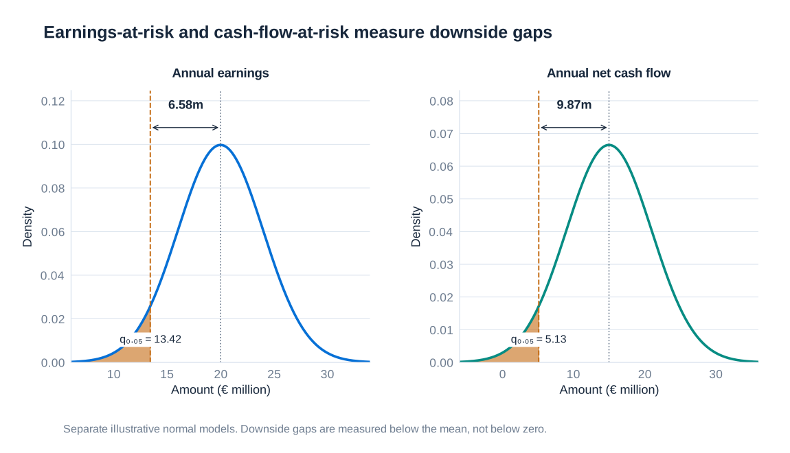
The example assumes separate marginal distributions and makes no claim about their correlation. The larger CFaR is consistent with cash being more sensitive to timing and financing shocks than earnings. The lower cash-flow quantile remains positive; the €9.87 million figure is a shortfall from the mean, not a €9.87 million cash loss. Normality is a teaching assumption and can miss asymmetric losses, defaults and discrete collateral triggers.
A terminal annual cash figure also cannot establish that every payment can be met during the year. A firm may finish December with positive cumulative cash after becoming unable to pay in June. Accordingly, cash-flow simulation should retain intermediate dates, currency needs, accessible reserves and committed funding. Stress scenarios complement quantiles by examining severe combinations that a fitted distribution may underrepresent.
Central-bank profits, gold and valuation reserves
Central banks illustrate why reported profit volatility cannot be read as a complete ranking of economic risk. The following historical figures show large fluctuations in Swiss National Bank results alongside a more stable sequence for the Bundesbank. They are rounded historical observations in different currencies, not a size-adjusted performance comparison or a forecast.
| Year | Bundesbank, EUR billion | Swiss National Bank, CHF billion |
|---|---|---|
| 2013 | 4.6 | −9.1 |
| 2014 | 2.95 | 38.3 |
| 2015 | 3.2 | −23.3 |
| 2016 | 0.4 | 24.5 |
| 2017 | 1.9 | 54.4 |
| 2018 | 2.4 | −14.9 |
| 2019 | 5.8 | 48.9 |
| 2020 | 0 | 21 |
For 2019, the SNB reported CHF 40.3 billion of profit on foreign-currency positions, CHF 6.9 billion of valuation gains on gold and CHF 2.1 billion on Swiss-franc positions, before the remaining items in the overall result. These components explain the rounded description of roughly 40, 7 and 2 billion. The historical comparison of gold holdings, approximately 3,374 tonnes for the Bundesbank and 1,040 tonnes for the SNB, is a dated stock comparison rather than a statement of current holdings.
Accounting treatment is crucial. The Bundesbank values gold at market prices; it does not simply retain gold forever at historical purchase cost. Unrealised gains are allocated to revaluation accounts rather than immediately included in annual profit. Unrealised losses first absorb the corresponding revaluation balance, with any excess treated under the applicable accounting rules. Consequently, a gold-price movement can change the balance-sheet valuation without producing the same movement in reported annual profit.
The 1997 German debate often called “Operation Goldfinger” concerned recognising and distributing gains associated with gold revaluation. Its enduring lesson is that a higher valuation is not a cash receipt, and neither automatically establishes a distributable profit. Differences in mandates, asset composition, currencies, balance-sheet size and recognition rules must be considered before attributing profit volatility solely to investment skill or risk appetite.
The SNB’s first three quarters of 2022 provide a further example: its reported loss was CHF 142.4 billion, including CHF 141.0 billion on foreign-currency positions. This is an interim result, not the full-year figure. Interest-rate, equity-price and exchange-rate movements can overwhelm coupon and dividend income without representing an equivalent immediate cash payment.
A gold hedge could reduce some economic exposure, but it might create derivative collateral needs and interfere with the purpose of holding reserves. Changing the accounting appearance alone is not a sufficient justification. Central-bank policy responsibilities also mean that private-sector profit maximisation is not an appropriate standalone objective.
Historical context and valuation checks: SNB annual result for 2019; SNB interim result at 30 September 2022; and the Bundesbank’s explanation of balance-sheet risks and revaluation accounts.
When a successful economic hedge produces an earnings loss
A reported interview with Bauer’s finance management in November 2019 describes interest-rate hedging instruments with a ten-year term and a fixed rate of 1%. Falling market rates subsequently produced a negative fair value and a charge in the quarterly accounts. The purpose described was to stabilise future borrowing costs. Calling the instrument unsuccessful solely because its own value fell misses the exposure it was intended to offset.
In the standard version of this strategy, floating-rate borrowing is combined with a pay-fixed, receive-floating interest-rate swap. If the borrowing pays reference rate plus spread , and the swap pays fixed rate while receiving , the combined annualised rate is approximately . This assumes matching reference rates, notionals and payment dates. The credit spread and any mismatch remain outside the simple hedge.
When market rates fall, the borrower’s future floating payments become cheaper, while the existing obligation to pay the swap’s fixed rate becomes less attractive. The swap’s negative market value can therefore accompany a reduction in the underlying funding cost. If the accounting timings differ, the derivative loss may appear before the corresponding future interest benefit. Qualification for hedge accounting cannot be assumed, and collateral requirements must be examined separately from the earnings presentation.
Hedging undeveloped reserves and choosing the right constraints
Consider a hypothetical oil producer such as Exxon acquiring an undeveloped field containing an assumed five million recoverable barrels. In a deliberately simplified undiscounted calculation, a USD 1 increase in the oil price raises gross reserve value by USD 5 million. The actual field value also depends on extraction costs, investment, production timing, taxes, recoverable quantities and discounting. The calculation describes a price sensitivity, not a complete valuation.
A short oil-futures position can offset part of the loss from falling oil prices. However, if oil prices rise, the futures position loses value and may require immediate variation-margin payments. The field’s offsetting increase in value does not provide cash while production has yet to begin. A hedge that reduces long-run price exposure can therefore create a near-term financing problem.
An additional mismatch arises if the field remains recorded on a cost basis while changes in the derivative enter current earnings. Economic gains in the reserves may not be recognised at the same time as derivative losses. Suitable hedge accounting, when its requirements are met, can address some recognition mismatches, but it does not manufacture cash or remove uncertainty about future production. Futures maturities and oil grades may also differ from the timing and quality of the eventual output.
A sound hedging decision therefore specifies a hierarchy of constraints: payments must be fundable; essential liabilities must be covered; economic losses must remain tolerable; and reported earnings must be understood under the applicable rules. Regulatory capital requirements under banking or insurance frameworks influence the cost of a position, but a reduction in required capital is not automatically an equal reduction in every economic risk. Likewise, a higher return on equity produced by a smaller equity denominator must be assessed alongside resilience.
The final decision should be made on the combined exposure and hedge, under both ordinary and adverse conditions. Compensation arrangements, earnings targets and accounting classifications can affect the choice, so governance should make those influences explicit. A useful risk report places market-value changes, earnings effects and dated cash requirements beside one another and explains which objective each proposed hedge serves.
10. Liquidity Risk
Being valuable is different from being able to pay
Liquidity is the ability to meet obligations when they fall due without incurring unacceptable losses. An institution needs the right amount of cash, in the right currency, in the right legal entity and before the relevant deadline. Assets with substantial long-term value cannot pay today’s creditor unless they can be sold, pledged or otherwise converted into usable funds in time. This is why a profitable business, or even one with assets worth more than its liabilities, can encounter a liquidity crisis.
Funding liquidity risk is the risk of being unable to obtain cash needed for payments, collateral calls or refinancing. Market liquidity risk is the risk that an asset cannot be sold or financed promptly at a price close to its undisturbed value. The two risks interact: an inability to refinance can force an asset sale, while the discount on that sale can worsen the institution’s financial position and undermine creditors’ willingness to lend.
Solvency concerns the capacity of asset value and future earnings to cover liabilities. Liquidity concerns the timing and accessibility of payment resources. The distinction is analytically useful, but crises rarely remain neatly separated. Credit losses can cause lenders to withdraw funding; a funding crisis can then generate fire-sale losses large enough to threaten solvency. Liquidity analysis should therefore incorporate both confidence shocks and deterioration in the underlying business.
How financial institutions produce and consume liquidity
Commercial banks provide customers with liquid deposits while financing assets such as mortgages and business loans that cannot all be realised immediately at their carrying value. They also promise liquidity through credit lines and other commitments. This maturity and liquidity transformation is economically useful, but it requires buffers, diversified funding and credible access to additional resources. A customer’s right to withdraw or draw a facility can become the bank’s cash obligation at an inconvenient moment.
Investment banks and securities dealers provide market liquidity by quoting prices and temporarily holding inventories. They also consume liquidity when they finance those inventories, meet margin calls, underwrite securities or bridge a client’s financing. An underwriting plan may assume that securities will be sold quickly; if demand disappears, the intermediary must finance an unwanted inventory for longer than expected. A securitisation pipeline can similarly leave loans or asset-backed securities on the balance sheet when distribution stops.
Funding diversity must be assessed by economic behaviour, not merely by counting contracts. Several lenders may all withdraw because they use the same collateral standard, credit rating or money-market signal. Geographic diversity does not help much if every funding source depends on the same securitisation market remaining open. Concentration by provider, instrument, currency, maturity and collateral type therefore matters.
Cash-flow gaps and survival horizons
A cash-flow ladder assigns expected receipts and payments to time buckets. For bucket , let be cash inflows, cash outflows and the net gap. With initially available cash , the projected balance before additional financing is:
All terms must use the same currency and units. Contractual maturity is the starting point, but behavioural assumptions are necessary for deposits, early repayments, option exercise and facility drawdowns. An expected refinancing is not equivalent to cash already available, particularly under stress. Intraday settlement obligations may require a finer time grid than a daily or weekly forecast.
| Time bucket | Inflows | Outflows | Net gap | Projected cash before new financing |
|---|---|---|---|---|
| Days 1–7 | 20 | 30 | −10 | 15 |
| Days 8–14 | 15 | 35 | −20 | −5 |
| Days 15–30 | 40 | 20 | 20 | 15 |
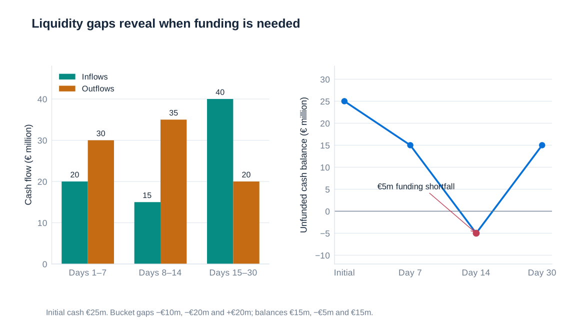
The end-of-month balance is positive, yet the institution has an unfunded €5 million gap by day 14. It needs at least that amount of additional accessible funding by the relevant payment dates; a prudent plan would also allow for uncertainty and any minimum operating cash requirement. The later €40 million inflow cannot retrospectively settle an earlier missed payment. A negative projected balance is a signal that the assumed plan is infeasible without intervention, not a literal balance that can be spent.
A survival horizon identifies how long the institution can continue meeting payments under a specified stress using resources that remain available. It is conditional on assumptions about deposit runoff, collateral haircuts, asset-sale capacity and committed facilities. Stress tests should combine institution-specific pressures with market-wide disruption, because the same event can reduce inflows, increase outflows and make asset sales more expensive.
Measuring market liquidity and collateral capacity
A narrow bid–ask spread indicates a small quoted transaction cost for a specified trade size. Market depth describes how much can be traded without moving the price substantially. Resilience describes how quickly the market absorbs an order imbalance and recovers. Trading volume is useful context, but heavy volume during distressed selling does not necessarily indicate that a large position can be sold cheaply. Executable prices, settlement constraints and the institution’s own position size matter.
Secured funding converts collateral into borrowing capacity. If collateral has market value and the lender applies haircut , a simplified borrowing limit is . The haircut is the fraction of collateral value excluded from the advance. It is not a general definition of the borrower’s accounting equity, although the unfunded part of the position must be financed through other resources.
Consider an explicitly hypothetical repo position. Collateral worth €100 million with a 10% haircut supports €90 million of borrowing. After its price falls to €95 million and the haircut rises to 25%, borrowing capacity becomes:
The borrower must find €18.75 million to repay funding or provide acceptable additional collateral, ignoring interest and other contractual details. This cash requirement is much larger than the €5 million asset-price decline. If the position initially contained €10 million of the borrower’s own funds and no other exposures, its remaining economic equity would still be €5 million before liquidation costs. Positive equity therefore does not by itself solve the immediate funding problem.
Liquidity spirals and the limits of short-term financing
A liquidity spiral arises when worsening market and funding conditions reinforce each other. Lower collateral prices reduce borrowing capacity; larger haircuts intensify the shortfall; borrowers sell assets to raise cash; selling pressure lowers prices further. Dealers facing the same constraints may reduce their capacity to absorb sales. Individually rational attempts to preserve liquidity can therefore worsen conditions for the system as a whole.
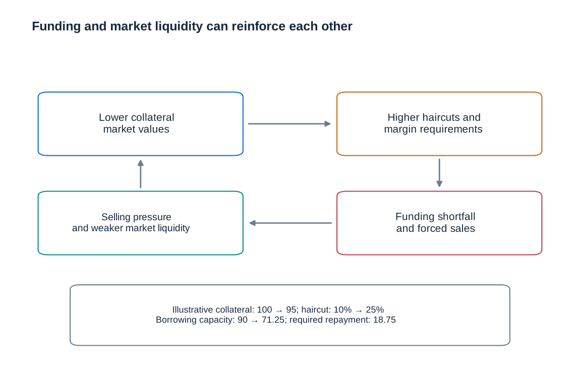
Brunnermeier and Pedersen’s analysis of market and funding liquidity formalises this interaction. The practical implication is that a haircut and an asset price should not always be stressed independently: both may deteriorate together. Collateral that seemed ample in normal markets may support much less borrowing when financing is most needed.
Lehman Brothers illustrates the vulnerability associated with substantial short-term secured funding and confidence-sensitive counterparties. Overnight or very short refinancing makes the institution repeatedly dependent on a fresh lending decision. Its failure cannot be reduced to one haircut or one liquidity mechanism: asset quality, leverage, valuation uncertainty, solvency concerns and counterparty confidence interacted. The general lesson is that a funding plan dependent on uninterrupted rollover needs severe tests of market closure and collateral deterioration.
Northern Rock: wholesale disruption and a retail run
Northern Rock’s 2007 experience shows why the visible queue outside a bank is not necessarily the beginning of the funding problem. Its mortgage business relied heavily on wholesale funding and securitisation. When those markets became difficult to access, the bank sought central-bank liquidity support. Retail withdrawals then intensified the pressure after the support became public.

A depositor who believes others will withdraw may want to withdraw first, because a bank cannot immediately convert its entire loan portfolio into cash without loss. This coordination problem can amplify concerns about a bank even when the initial disturbance comes from wholesale markets. Deposit protection, credible public communication and access to liquidity can influence that behaviour, but none substitutes for a funding structure able to withstand disruption.
The case also illustrates the difference between a solvent asset portfolio under orderly collection and the resources needed to meet rapid withdrawals. On 14 September 2007, the Bank of England announced a support facility against appropriate collateral at a premium interest rate. Analysing the episode requires attention to the wholesale funding model and the subsequent retail run together, rather than treating the photograph of depositors as a complete explanation.
Historical sources: the Bank of England’s Northern Rock liquidity-support announcement and the UK Treasury Committee’s inquiry into the bank’s funding model. The feedback mechanism is developed in Markus K. Brunnermeier and Lasse Heje Pedersen (2009), Market Liquidity and Funding Liquidity.
Contingent funding: IKB and AIG
Liquidity commitments can transmit stress from an apparently separate vehicle to its sponsoring bank. IKB’s involvement with the Rhineland Funding conduit illustrates the mechanism. The vehicle financed longer-lived asset-backed exposures using short-term asset-backed commercial paper. If investors refused to roll that paper, a committed liquidity facility could be drawn, transferring an immediate funding requirement to the bank.
The commitment resembles a contingent promise to absorb assets or provide cash when market financing becomes unavailable. The analogy to a written put is useful because the obligation tends to become costly in adverse states. It is not an assertion that every liquidity facility has the same payoff as a simple traded put: draw conditions, collateral eligibility, credit exclusions and recourse depend on the actual contract. Exposure analysis must read those terms and consider correlated drawdowns across facilities.
AIG provides a related but distinct mechanism. Credit protection sold on structured-credit exposures created obligations that depended on collateral agreements as well as eventual credit events. Falling valuations and rating-related triggers could generate collateral calls before the reference assets suffered final default losses. Cash therefore became necessary on a timetable different from the eventual insurance or credit-loss settlement.
This distinction prevents two errors. A margin call does not by itself establish the ultimate loss on the underlying asset, but neither can it be dismissed merely because that loss has not yet occurred. Counterparty agreements, downgrade provisions, eligible collateral and the ability to obtain cash must be incorporated into stress tests. A position described as remote from expected default can still have demanding liquidity consequences.
Pension hedges and the 2022 gilt-market disruption
Liability-driven investment seeks to manage the sensitivity of pension assets relative to promised benefits. A pension liability resembles a stream of long-dated payments, so its present value generally rises when discount rates fall. Receiving a fixed rate and paying a floating rate in an interest-rate swap can add asset-side interest-rate sensitivity and help hedge that liability exposure without buying the full notional amount of bonds.
For a hypothetical illustration, take a scheme with £100 million of liabilities, £20 million in gilts and £80 million in illiquid private-equity investments. Suppose it also enters a receive-fixed, pay-floating swap with £80 million notional. The swap notional is a reference amount for payments and sensitivity; it is not an additional £80 million asset to add to the balance sheet. At inception, a market-rate swap can have approximately zero value.
If yields rise sharply, the gilts and the receive-fixed swap lose value. The present value of pension liabilities can fall too, so the scheme’s long-run funding position need not deteriorate in the same way as its immediate cash position. The lower liability valuation, however, delivers no cash with which to meet the swap’s collateral call. Private-equity holdings may not be saleable quickly, leaving gilts or other liquid assets as the immediate source of funds.
During the September 2022 UK gilt-market disruption, distressed selling by liability-driven investment funds reinforced falling prices and collateral pressure. The Bank of England introduced temporary, targeted gilt purchases to restore market functioning and allow time for adjustment. The case demonstrates that a hedge of long-term liability value needs a separately funded collateral buffer. The asset allocation and numbers above explain the mechanism; they are not a reconstruction of every affected fund.
The historical mechanism and intervention are described by the Bank of England in Financial stability buy/sell tools: a gilt market case study (2023).
Metallgesellschaft: a long-term hedge with short-term cash demands
Metallgesellschaft’s 1993 difficulties illustrate a similar timing problem in commodity markets. Long-term commitments to deliver oil products at fixed prices created exposure to rising oil prices. Long positions in shorter-dated oil futures could offset part of that exposure: higher oil prices would increase the cost of supplying customers but generate gains on the futures.
When oil prices fell, the futures generated losses and cash margin requirements. The fixed-price delivery commitments became economically more favourable, but that benefit was embedded in future deliveries rather than immediately available cash. Maintaining the hedge therefore required financing the interval between derivative losses and the realisation of offsetting operating benefits.
A one-for-one match in barrel quantities is not automatically a perfect hedge. Futures maturity, the shape of the forward curve, roll costs, product quality, customer performance and the timing of deliveries all matter. The case should consequently not be interpreted as proof that an otherwise riskless strategy failed solely because managers misunderstood margin. Its broader lesson is that economic hedging, basis risk and the funding of intermediate cash flows must be evaluated jointly.
Central-bank access and foreign-currency liquidity
Central-bank funding is conditional on eligible counterparties, acceptable collateral and the governing operational rules. In February 2015, the ECB removed the waiver that had allowed certain Greek sovereign-issued or guaranteed instruments to serve as collateral despite not meeting normal minimum credit-rating requirements. This did not remove Greek banks’ counterparty status or mean that every channel of central-bank support ceased. The ECB explained that relevant national-central-bank emergency liquidity assistance could address needs within the applicable rules.
The distinction matters for a contingency plan. An asset may retain economic value while becoming ineligible in a particular facility. Funding capacity then changes even without an immediate contractual default. Available collateral, operational readiness and the conditions attached to alternative facilities should be mapped in advance; emergency assistance must not be modelled as unconditional private funding.
Currency creates another constraint. A European bank holding dollar assets cannot necessarily finance a dollar payment with euro cash at an acceptable cost during a dollar shortage. It may depend on dollar wholesale borrowing or on rolling foreign-exchange swaps. Those channels introduce refinancing and cross-currency basis risk, even where the long-term currency exposure is hedged.
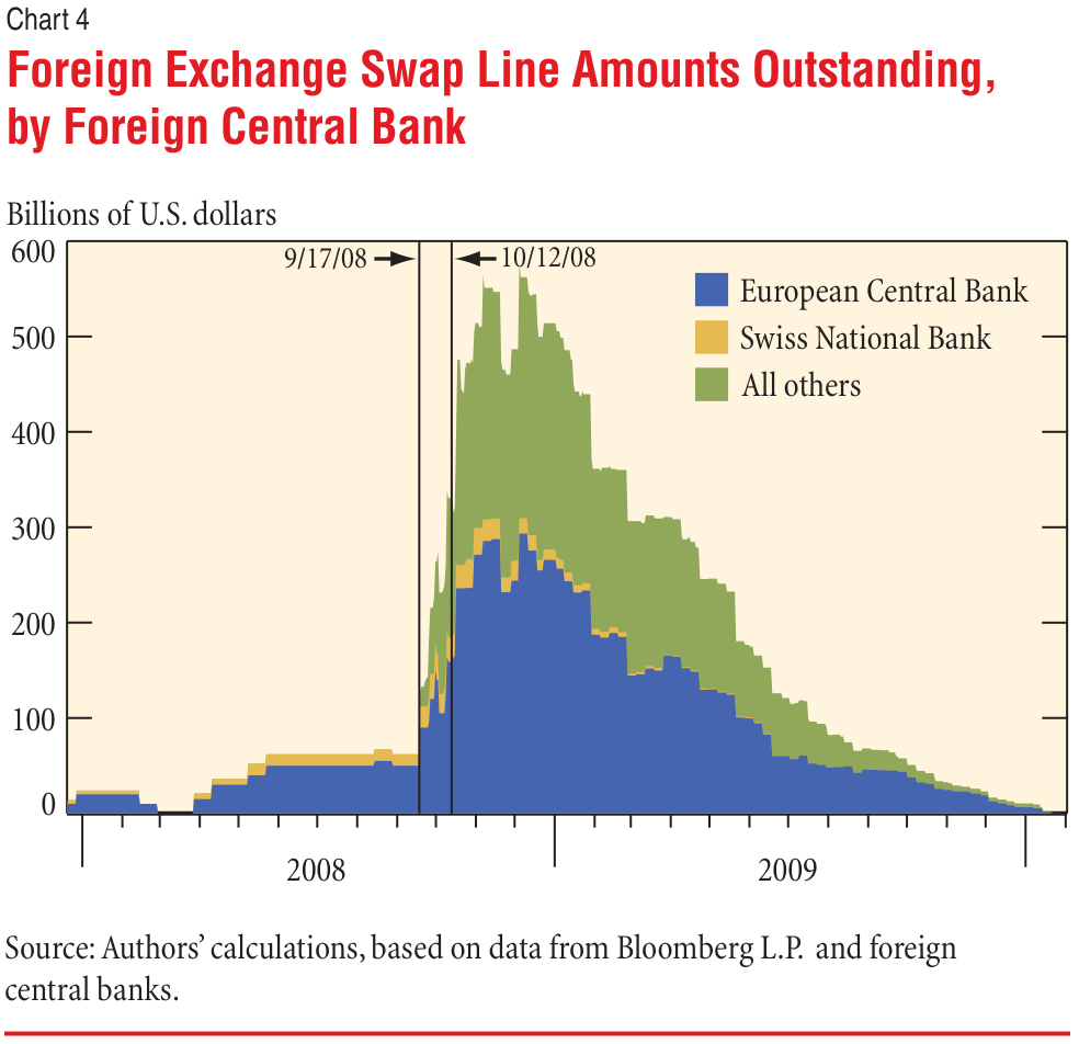
Central-bank swap lines address this currency-specific shortage by enabling a foreign central bank to obtain dollars from the Federal Reserve and provide dollar liquidity in its jurisdiction. The historical expansion of such arrangements during the financial crisis reflects strains in international dollar funding. The figure records that historical episode; it should not be read as a forecast or as a statement that every institution has direct access to the Federal Reserve.
Primary sources: ECB, Eligibility of Greek bonds used as collateral in Eurosystem monetary policy operations (4 February 2015), Federal Reserve, Central bank liquidity swaps; and Michael J. Fleming and Nicholas J. Klagge (2010), The Federal Reserve’s Foreign Exchange Swap Lines, Chart 4.
The Liquidity Coverage Ratio and a usable stress buffer
The Basel Liquidity Coverage Ratio, or LCR, compares a stock of qualifying high-quality liquid assets with net cash outflows in a specified 30-calendar-day stress scenario. Under normal conditions, the minimum ratio is 100%:
Here HQLA is the eligible liquid-asset stock after applicable adjustments, and is stressed net outflow over 30 days. The buffer is intended to be used during stress. Basel explicitly allows the ratio to fall below 100% in such circumstances, with supervisory assessment and response reflecting the situation. Treating every stress-time use of the buffer as automatically impermissible would undermine its purpose.
HQLA must meet asset-quality and operational conditions, including availability for monetisation. Nominal ownership is insufficient if an asset is encumbered or cannot be mobilised by the liquidity-management function. Level 1 assets face no overall composition cap; Level 2 assets are limited to 40% of the qualifying stock, and Level 2B assets to 15%, subject to the framework’s adjustments. The relevant haircuts and caps mean that the accounting value of securities is not necessarily their HQLA amount.
Stressed outflows apply prescribed assumptions to funding withdrawals, commitments and other obligations. Eligible inflows are restricted, including an overall cap of 75% of outflows in the basic calculation. If is stressed outflow and eligible inflow before that cap, the simplified expression is:
Consider a hypothetical bank with €120 million of eligible HQLA, €160 million of stressed outflows and €60 million of eligible inflows. The cap is €120 million, so all €60 million of inflows are counted. Net outflows are €100 million and the LCR is , or 120%. The €20 million excess is a buffer above this particular regulatory requirement, not proof that every payment path or stress is covered.
If eligible inflows instead equal €140 million while outflows remain €160 million, the cap permits only €120 million to offset outflows. Net outflows are therefore €40 million rather than €20 million. The cap limits reliance on expected receipts and ensures a minimum holding of liquid resources relative to gross stressed outflows.
Regulatory sources: Basel Framework LCR20 on the minimum and stress-time buffer use, LCR30 on HQLA, and LCR40 on cash flows. Basel standards provide the international framework; jurisdictional implementation and institution-specific requirements must also be considered.
The Net Stable Funding Ratio
The Net Stable Funding Ratio, or NSFR, addresses the stability of the funding structure over a one-year horizon. It compares available stable funding, ASF, with required stable funding, RSF. Funding categories receive weights reflecting their expected stability; assets and selected off-balance-sheet exposures receive weights reflecting their funding needs:
Here denotes a funding amount, including eligible capital; is its ASF factor. The amount and factor describe an asset category, while captures relevant off-balance-sheet requirements. The factors are regulatory weights, not forecasts that an identical fraction will certainly leave or remain. The NSFR is a structural measure and does not replace a dated cash forecast.
| ASF factor | Representative qualifying funding |
|---|---|
| 100% | Eligible regulatory capital and qualifying funding with effective residual maturity of at least one year |
| 95% | Qualifying stable retail and small-business demand deposits or deposits with residual maturity below one year |
| 90% | Corresponding less stable retail and small-business deposits |
| 50% | Non-financial corporate funding below one year; certain other funding from six months to below one year |
| 0% | Funding outside the qualifying categories, including ordinary very short-term financial-institution funding |
Deposit classification matters: the 95% and 90% factors are distinct from the lower weights in early versions of the international liquidity proposals. “Stable” is a defined regulatory category, not an informal judgement that a customer seems loyal. Effective maturity, early-withdrawal rights and the identity of the provider can affect classification.
| RSF factor | Representative qualifying asset or exposure |
|---|---|
| 0% | Cash and central-bank reserves |
| 5% | Unencumbered Level 1 assets other than cash and central-bank reserves |
| 10% | Qualifying financial-institution loans below six months, secured by reusable Level 1 collateral |
| 15% | Unencumbered Level 2A assets and certain other financial-institution loans below six months |
| 50% | Unencumbered Level 2B assets and qualifying shorter-term non-financial loans |
| 65% | Qualifying unencumbered residential mortgages of at least one year with standardised risk weight no greater than 35% |
| 85% | Other qualifying performing long-term non-financial loans; physical commodities including gold; derivative initial margin |
| 100% | Fixed assets, non-performing loans and assets encumbered for at least one year |
| 5% of undrawn amount | Irrevocable and conditionally revocable credit and liquidity facilities |
The tables give representative categories, not a complete substitute for the rules. A short maturity alone does not give every loan a zero RSF factor. Encumbrance, counterparty type and derivative treatment can change the requirement. Undrawn commitments also matter because they can require funding after a customer exercises the right to draw.
For a hypothetical €100 million balance sheet, suppose assets consist of €10 million cash, €20 million qualifying unencumbered Level 1 securities and €70 million qualifying mortgages in the 65% category. Funding consists of €10 million eligible capital, €50 million stable qualifying deposits in the 95% category and €40 million ordinary financial-institution borrowing with maturity below six months and a 0% factor. Ignoring other exposures:
Both assets and funding total €100 million, but the weighted amounts differ. Passing the ratio does not eliminate the need to refinance the €40 million borrowing or meet deposit withdrawals. The example demonstrates the distinction between a structural regulatory test and a complete survival analysis.
Regulatory sources: Basel Framework NSF20 on the ratio, NSF30 on ASF and RSF definitions, and NSF99 for category summaries.
Turning measurements into a contingency funding plan
The LCR examines a specified short stress, while the NSFR disciplines structural funding. A bank can satisfy both and remain exposed to a concentrated payment, an unavailable currency, an operational barrier or a shock beyond their assumptions. Internal cash ladders, collateral inventories and stress tests should therefore supplement regulatory ratios.
A contingency plan connects observable warning signals to actions that can actually be executed. Signals can include rapid deposit outflows, widening funding spreads, larger haircuts, rating changes and declining collateral capacity. Responses might involve drawing genuinely available committed lines, mobilising prepositioned collateral, obtaining longer funding, reducing positions or slowing new commitments. Each action needs an owner, a realistic execution time and an estimate of its effect on counterparties and markets.
Plans must avoid double counting. The same security cannot simultaneously fund an asset sale and remain pledged to support existing borrowing. A facility cannot be treated as unconditional if a covenant or adverse-change clause could prevent drawing. Transfers between subsidiaries may face legal or operational barriers, and an assumed sale price must reflect the size of the position under stress.
Liquidity risk management ultimately combines balance-sheet design with preparation for adverse timing. It asks how a business model supplies liquidity to others, when those promises become cash obligations, and which resources remain usable when confidence falls. Economic hedges, accounting profit and regulatory compliance all contribute information, but the decisive operational question remains whether every due payment can be funded on time.
Appendix A. Core Formula Reference and Variable Definitions
The following equations collect the most frequently used formulas in this manual. Conventions can change across contexts: always specify the risk horizon, return or yield convention, direction of the exposure, and definitions of loss and recovery.
Introduction, Risk Governance and Stock-Market Risk
The weights wᵢ represent capital proportions; covariance determines whether risks amplify or offset one another.
L is loss, defined as minus profit and loss; it may be negative when there is a gain. The confidence level α specifies the cumulative probability used to locate the quantile.
ES quantifies the average severity of losses in the tail; for discrete distributions a generalized tail mean definition is necessary.
A first-order one-period exposure formula: LGD is a loss fraction, and EAD is the exposure amount at default.
Capital is set aside for losses above average expected losses up to the stated tail quantile.
Expected return is linear in portfolio weights; risk is not.
Σ is the covariance matrix of individual security returns; w is the vector of portfolio weights.
For a one-period linear portfolio with normally distributed return: V₀ is value, μp return mean, σp return standard deviation, zα the standard-normal α quantile.
Beta measures portfolio sensitivity to a representative market index.
The minus sign denotes selling the index future to offset the positive market beta of long equities.
μ is instantaneous expected proportional drift; σ is volatility; W is a standard Brownian motion.
The drift correction −σ²/2 appears when simulating continuously compounded stock returns.
Expected return in excess of the risk-free rate per unit of total portfolio volatility.
Excess expected return per unit of systematic market exposure.
Foreign Exchange Risk and Corporate Hedging
Check the direction of the exchange-rate quotation before translating; inverse quotes require division.
The approximation is exact when q is home currency per foreign currency and the foreign-currency cash amount X stays fixed.
With an exchange rate quoted as home currency per unit of foreign currency and continuously compounded funding rates , covered interest parity gives
The formula assumes matching maturities and conventions and frictionless access to the relevant funding and forward markets. Actual quotations may reflect a cross-currency basis and transaction costs.
Commodity Price Risk and Minimum-Variance Hedging
Sᵀ is the spot price at maturity; F₀,T is the delivery price contracted today.
Applies with continuous compounding, freely tradable underlying and no distributions or storage effects.
r financing rate, u storage cost rate, y convenience yield, T time to delivery.
Minimizes Var(ΔS + NΔF) for a linear hedge. Here ΔS is the monetary change of the entire exposure and ΔF the monetary change of one futures contract; using prices per unit instead requires adjustment for exposure quantity and contract size.
The regression slope of exposed value changes on futures changes gives hedge size with the opposite sign.
ρSF is the correlation of hedged exposure and futures value changes; R² measures the fraction of variance eliminated.
Interest Rate Risk, Duration and Banking-Book Exposure
F face value, y effective annual yield to maturity, T years to maturity.
Each payment time is weighted by its share of the bond price.
Discrete annually compounded convention; for other compounding conventions adjust the denominator accordingly.
C is price convexity, defined with a consistent yield convention; Δy is a decimal yield change.
PVBP (also DV01) is approximately the price loss from a one-basis-point yield rise for a positive-duration bond.
Under a normal-yield-shock and first-order duration model, use σ measured in basis points.
A and L denote present values of banking-book assets and liabilities; D terms their relevant effective duration.
Option-Related Risks and Greeks
Subtract the premium from the payoff to compute buyer profit; the seller receives the opposite payoff plus premium.
Assumes K₁ < K₂; the net premium is the lower-strike call cost less higher-strike call proceeds.
A long call and long put with a common strike generate a V-shaped terminal profit profile.
This is a local Taylor approximation. Here theta measures sensitivity to elapsed calendar time, volatility and rates are expressed as decimal inputs, and monetary exposures require position quantities. Higher-order and cross-effects may matter for large shocks.
Delta gives local exposure to underlying price; gamma is the change of that exposure with underlying price.
Sensitivity definitions rely on the pricing model and exact time/rate units.
Value at Risk Models and Market-Risk Measurement
α confidence level and h holding period specify the loss distribution being quantified.
With positive loss defined as negative P&L; sign convention for the mean must be checked.
Each Li is the loss after repricing the current holdings under a historical risk-factor scenario.
Generate M risk-factor paths or shocks and reprice the current portfolio in each scenario.
a contains portfolio P&L sensitivities to risk-factor shocks; Σ is their covariance matrix. This form assumes a zero P&L mean; otherwise subtract the expected P&L.
A complementary tail-risk statistic, particularly relevant when extremely bad outcomes are far beyond the VaR threshold.
The integral form of Expected Shortfall includes exactly the worst fraction of outcomes and remains valid for distributions with probability masses:
Here ranges over confidence levels, and the denominator is the tail probability. A simple conditional average above VaR can omit part of the boundary probability mass in a discrete distribution.
For a normal profit-and-loss variable with mean and standard deviation , the normal loss measures are
is the standard-normal quantile and its density. The normal-tail assumption is substantive: neither expression establishes that realised losses will be normally distributed.
The univariate EWMA forecast and a GARCH(1,1) specification are respectively
is the return innovation. For EWMA, controls memory; in a conventional stationary GARCH model, , and . These describe conditional variances, not a guarantee of normally distributed shocks.
Credit Risk, Ratings, Regulatory Capital and Portfolio Models
Separate probability of default from loss severity and the amount exposed at default.
The 12.5 factor equals the inverse of an 8% minimum total capital ratio; actual IRB computations include regulatory correlations, maturity adjustments and other adjustments.
Risk-neutral default probabilities are inferred from market prices, recovery assumptions and discount factors.
A price-implied risk-neutral default probability is generally not identical to the historical or physical probability of default.
xᵢ are measurable credit-quality variables; βᵢ are weights estimated or chosen by a credit modeller.
The logistic link maps a linear score to a probability between zero and one.
For a receiver operating characteristic (ROC) curve with default as the positive class, AUC is the area under that curve. This Gini expression must not be applied to the unnormalised area under a cumulative accuracy profile (CAP).
An institution needs credit portfolio scenarios to model dependence and extreme co-defaults.
A conditional annual default probability follows from cumulative default probabilities :
The denominator is the probability of surviving to the start of year . Cumulative and conditional probabilities should not be added or compared as if they represented the same horizon and population.
Credit Default Swaps and Asset-Backed Securities
A spread of 90 bps equals 0.90% annually; the actual timing and accrual depend on the contract.
Simplified cash settlement on a full notional N, ignoring accrued amounts and contractual nuances.
A is attachment point, D detachment point and Lpool total pool loss expressed in matching units.
Earnings at Risk and Cash Flow at Risk
C is constant annual cash coupon and r the discount yield. A change in r changes price even when C stays constant.
The expression gives the coupon rate. Multiply by notional and the accrual fraction to obtain a cash coupon. Frequent resets reduce rate-driven price exposure but make future coupon cash flows variable.
Liquidity Risk and Basel Liquidity Requirements
A standardized short-term liquidity stress measure; the general regulatory minimum is 100%.
Measures the extent to which asset and off-balance-sheet financing needs are supported by sufficiently stable funding; general minimum 100%.
For an LCR calculation with the standard 75% inflow cap, qualifying stressed outflows and inflows give
is the regulatory 30-day net cash outflow. Eligibility rules, haircuts, caps and permitted exceptions determine which amounts enter the calculation; this identity does not replace those rules. Both the liquidity buffer and the cash-flow amounts are measured in the same currency.
Appendix B. Glossary of Financial Risk Terms
This glossary gives concise definitions for consultation. The chapters explain the assumptions, calculations and limitations behind each term.
A–D
- Accrued premium
- CDS premium earned since the previous payment date but not yet paid. Settlement after a credit event can require accrued premium in addition to the protection payment.
- Adverse selection
- A situation in which information asymmetry makes the counterparties most willing to accept a contract systematically different from those a naive model assumes.
- Asset liquidity
- Ease and cost of turning an asset into cash through sale or secured financing.
- Asset-backed security (ABS)
- A security whose contractual cash flows depend on a pool of underlying receivables or other financial assets, often issued through an SPV and divided into tranches.
- Backtesting
- Comparison of model forecasts with realised outcomes using a consistent portfolio, horizon and loss definition. Exception frequency alone does not test every aspect of a risk model.
- Backwardation
- A term structure in which longer-dated forward or futures prices are below nearer-dated prices. A downward curve is not a guarantee that the future spot price will fall.
- Banking book
- Bank positions outside the regulatory trading book, commonly including lending and deposits. Accounting classification and regulatory book allocation are distinct decisions.
- Basis point
- One hundredth of a percentage point: 1 bp equals 0.01%, or 0.0001 as a decimal rate change.
- Basis risk
- Risk that movements in a hedge instrument do not closely match the hedged exposure.
- Beta
- Sensitivity of a portfolio return to the return of a reference market index.
- CAP curve
- Cumulative accuracy profile: cumulative share of defaults captured as borrowers are examined from highest to lowest predicted risk. It differs from the receiver operating characteristic curve.
- Capital at risk
- The amount of capital exposed to an adverse event, depending on the chosen risk framework.
- Cash Flow at Risk (CFaR)
- Adverse-tail quantile of projected actual cash flows relative to a forecast or benchmark.
- CDS
- Credit default swap: derivative transferring a specified credit-event exposure for a premium.
- Central counterparty (CCP)
- An entity that interposes itself between counterparties in eligible cleared transactions. Clearing changes counterparty risk and creates margin and liquidity requirements; it does not remove risk.
- Conditional default probability
- Probability of default during a specified interval conditional on survival to the beginning of that interval. It differs from cumulative default probability measured from origination.
- Contango
- A forward curve whose farther-dated contracts trade at higher prices than nearer-dated contracts.
- Convenience yield
- Economic advantage associated with physical possession of a commodity.
- Convexity
- Curvature of a bond price–yield relationship, improving on a duration-only approximation.
- Correlation
- Standardized measure of linear co-movement, bounded between −1 and +1.
- Covariance
- The expected product of deviations from two means, measuring linear co-movement in the original units of the variables. Portfolio variance combines every relevant covariance.
- Credit migration
- A change in assessed creditworthiness or rating grade short of outright default.
- Credit spread
- Yield increment over a specified benchmark, reflecting expected losses together with risk premia, liquidity and other pricing effects. It is not a direct physical default probability.
- Delta
- First derivative of option value with respect to underlying price.
- Detachment point
- Pool-loss threshold at which a tranche is completely exhausted. Its attachment point is the threshold at which the tranche first begins to absorb losses.
- Diversification
- Combining exposures whose losses are not perfectly aligned. Its benefit depends on dependence, concentration and the risk measure, and may weaken during stress.
- Duration
- Weighted bond cash-flow timing or price sensitivity, depending on specified definition.
- DV01 / PVBP
- Approximate monetary change in value for a one-basis-point parallel yield movement, with the quoted sign convention specified. For a positive-duration bond it is often reported as the magnitude of the loss from a yield rise.
E–H
- EAD
- Exposure at default, the amount owed or at risk when default occurs.
- Earnings at Risk (EaR)
- Adverse-tail sensitivity of reported accounting earnings.
- Economic capital
- Capital set to absorb unusually adverse losses above average expected loss.
- Economic FX exposure
- Sensitivity of future economic value or operating cash flows to exchange rates, including competitiveness, demand and input costs beyond existing contractual receivables.
- Economic value of equity (EVE)
- Present value of banking-book asset cash flows less liability cash flows under a stated valuation model. Its sensitivity need not have the same sign as near-term net interest income.
- EWMA
- Exponentially weighted moving average, a volatility updating rule that progressively reduces the weight assigned to older squared innovations.
- Expected Shortfall (ES)
- Average loss in the worst specified fraction of outcomes, using a quantile-integral definition that handles discrete probability masses consistently.
- Funding liquidity
- Capacity to raise cash or meet payment and margin obligations when due.
- Gamma
- Second derivative of option value with respect to underlying price.
- GARCH
- Generalised autoregressive conditional heteroskedasticity: a family of models in which conditional variance depends on past innovations and past variances.
- Geometric Brownian motion (GBM)
- A continuous-time price model with proportional drift and volatility. Its lognormal terminal distribution excludes price jumps and does not describe every asset or crisis regime.
- Haircut
- Discount to collateral market value used when determining secured funding.
- Hedge accounting
- An accounting framework that can align recognition of eligible hedging instruments and hedged items when designation and other requirements are satisfied. An economic hedge does not qualify automatically.
- Hedge ratio
- Amount of hedging instrument required to offset a chosen part of an exposure.
- Historical simulation
- Risk measurement by applying historical risk-factor shocks to the current portfolio and repricing. Historical portfolio returns and current-portfolio scenario losses need not be the same data.
- HQLA
- High-quality liquid assets, eligible assets in the LCR liquidity buffer.
I–P
- Initial margin
- Collateral collected to cover potential future exposure over a liquidation or close-out period. Its amount and eligibility can change as risk conditions change.
- IRRBB
- Interest rate risk in the banking book, including changes in economic value or net interest income.
- Leverage
- Exposure or assets relative to a specified capital base. Small asset-value changes can produce much larger percentage changes in equity when leverage is high.
- LGD
- Loss given default; default loss as a fraction of exposure after recovery.
- Liquidity Coverage Ratio
- Ratio of qualifying liquid assets to standardized stressed 30-day net outflows.
- Margin call
- A demand for additional cash or eligible collateral. An economically hedged portfolio may still face substantial interim funding needs.
- Mark-to-market
- Recognition or measurement by reference to current fair/market value.
- Merton model
- A structural credit model treating equity as a call option on firm assets and debt default as a consequence of asset value falling below the debt obligation at the model horizon.
- Model risk
- Risk of adverse decisions or losses caused by an incorrect, miscalibrated, misimplemented or misused model, including unreliable data and assumptions.
- Modified duration
- Approximate negative percentage bond price sensitivity per unit yield change.
- Monte Carlo simulation
- Numerical generation of scenarios under a specified stochastic model. More simulations reduce sampling error but do not repair a wrong model.
- Net interest income (NII)
- Interest income less interest expense over an accounting period. Repricing, customer behaviour, volumes and the term structure jointly determine its response to rate changes.
- NSFR
- Net Stable Funding Ratio, available stable funding divided by required stable funding.
- Operational hedging
- Changes in physical operations, financing, sourcing or production to reduce exposure.
- PD
- Probability that an obligor defaults within a specified horizon and definition.
Q–Z
- Repo
- Repurchase agreement, a form of collateralized short-term financing.
- Risk appetite
- The types and amounts of risk an institution is prepared to accept in pursuit of its objectives, translated into meaningful limits and governance responsibilities.
- Risk-neutral probability
- A pricing probability consistent with a specified no-arbitrage valuation model. It incorporates risk pricing and generally differs from an objective forecast of event frequency.
- Risk-weighted assets (RWA)
- Regulatory measure of exposures after capital-rule risk weight and model calculations.
- Rollover risk
- Risk that maturing funding cannot be renewed in the required amount or at an affordable price. Repeatedly replacing short hedges or funding can create rollover exposure.
- SPV
- Special-purpose vehicle holding transferred assets and issuing securities or other claims.
- Stress testing
- Evaluation of portfolio or business outcomes under specified adverse scenarios. A scenario can be informative without being assigned a precise probability.
- Systemic risk
- Risk of failure or destabilization propagating through the financial system.
- Theta
- Sensitivity of derivative value to elapsed calendar time or to remaining maturity. The chosen time convention determines the sign; it must be stated explicitly.
- Trading book
- Positions assigned to the regulatory trading book under applicable rules, generally involving trading intent or hedging of eligible trading positions. It is not synonymous with every fair-value accounting position.
- Transaction FX exposure
- Sensitivity of foreign-currency contractual/forecast transactions to exchange rates.
- Translation FX exposure
- Sensitivity of reporting-currency balance-sheet or consolidation numbers to exchange rates.
- Unexpected loss
- Severe credit-loss risk above expected loss; definitions vary across models.
- VaR
- Value at Risk: a loss-distribution quantile at a stated confidence level and horizon. Losses can exceed it, and it does not describe the severity of those exceedances.
- Variation margin
- Collateral transfers reflecting changes in the current market value of covered positions. Daily settlement can create immediate cash needs before gains elsewhere become available.
- Vega
- Sensitivity of an option’s value to a volatility input change.
- Wrong-way risk
- Dependence in which counterparty credit quality deteriorates when the exposure to that counterparty increases.
- Zero-coupon bond
- A debt instrument paying no interim coupon and a specified amount at maturity. Its price depends on the discount factor and the relevant credit and contractual assumptions.